Coupled temperature-displacement submodeling

This problem contains basic test cases for one or more Abaqus elements and features.

The following topics are discussed:

Elements tested
Features tested
Problem description
Results and discussion
Input files
Figures

ProductsAbaqus/StandardAbaqus/Explicit

Elements tested

SC8RT

C3D8HT
C3D8RHT
C3D8RT
C3D4T
C3D6T
C3D8T
C3D20HT
C3D20RHT
C3D20RT
C3D20T

CAX4HT
CAX4RHT
CAX3T
CAX4T
CAX4T
CAX6MHT
CAX6MT
CAX8HT
CAX8RHT
CAX4RT
CAX8RT
CAX8T

CGAX3HT
CGAX3T
CGAX4HT
CGAX4RHT
CGAX4RT
CGAX4T
CGAX6MHT
CGAX6MT
CGAX8HT
CGAX8RHT
CGAX8RT
CGAX8T

CPE4HT
CPE4RHT
CPE4T
CPE6MHT
CPE6MT
CPE8HT
CPE8RHT
CPE8RT
CPE3T
CPE4RT
CPE8T

CPEG3T
CPEG4RHT
CPEG4RT
CPEG4T
CPEG6MHT
CPEG6MT
CPEG8T

CPS4RT
CPS3T
CPS4T
CPS6MT
CPS8RT
CPS8T

Features tested

The submodeling capability is applied to two-dimensional, three-dimensional, and axisymmetric continuum coupled temperature-displacement elements. General steps invoking the steady-state coupled temperature-displacement and the dynamic temperature-displacement procedures are used in Abaqus/Standard and Abaqus/Explicit, respectively, for both the global and submodel analyses.

Problem description

Model:

All global models have dimensions 7.0 × 7.0 in the x–y or r–z plane. Each submodel has dimensions 5.0 × 5.0 in the x–y or r–z plane and occupies the lower right-hand corner of the corresponding global model. In all but the axisymmetric models, the out-of-plane dimension is 1.0. In axisymmetric models the structure analyzed is a hollow cylinder with an outer radius of 8.0.

Material:

In Abaqus/Standard:

Young's modulus	30 × 10⁶
Poisson's ratio	0.3
Coeff. of thermal expansion	1 × 10⁻⁵
Thermal conductivity	3.77 × 10⁻⁵
Specific heat	0.39
Density	82.9

In Abaqus/Explicit:

Young's modulus	110 × 10⁹
Poisson's ratio	0.3
Coeff. of thermal expansion	1 × 10⁻³
Thermal conductivity	390
Specific heat	384
Density	8900

Loading:

In all Abaqus/Standard models a distributed flux of magnitude 0.3 is applied to the right face; in Abaqus/Explicit the flux magnitude is 0.5× 10⁴.

Boundary and initial conditions

In the global model fixed boundary conditions $u_{1}$ =0 and $u_{2}$ =0 are prescribed on the left and bottom faces, respectively. In three-dimensional models the additional constraints $u_{3}$ =0 are applied to the nodes on the front and back faces. The initial temperature is zero everywhere, and fixed temperature boundary conditions are applied on the left face. In the submodel $u_{2}$ =0 is prescribed everywhere on the bottom face, while degrees of freedom 1, 2, and 11 for the nodes on the top and left faces are being driven by the global solution. The mass scaling technique is used in the Abaqus/Explicit models to speed-up the analysis.

Results and discussion

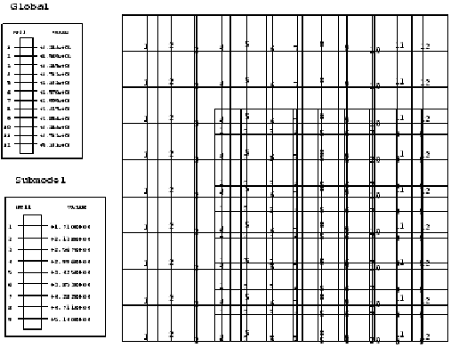
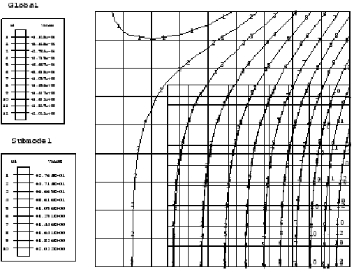
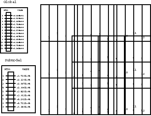
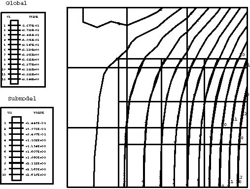
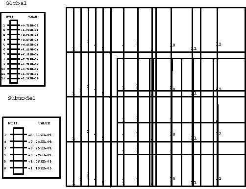
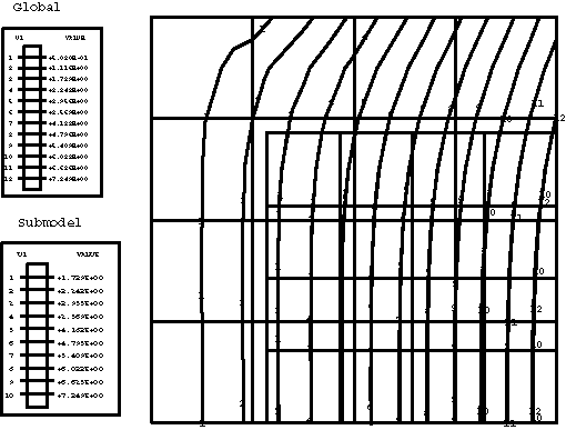
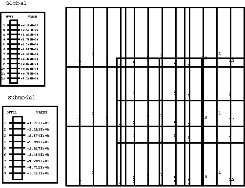
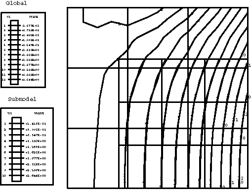
In the global analyses the temperature field predicted by Abaqus varies linearly in the x-direction in nonaxisymmetric models and logarithmically in the r-direction in axisymmetric models. The predicted displacement field is nonuniform in all models. The Abaqus/Standard results depicted for the temperature and x- or r-displacement contour plots are shown below. For comparison purposes the temperature and displacement solutions predicted by the submodels are also presented in the same contour plots, and excellent agreement between the global and submodel results is obtained. Hence, the amplitudes of all driven variables in the submodel analysis are identified correctly in the global analysis file output and applied at the driven nodes in the submodel analysis.

Global and submodel analyses results for 4-node plane stress elements in Abaqus/Standard are shown in Figure 1 and Figure 2.

Global and submodel Abaqus/Standard analyses results for 8-node plane strain elements are shown in Figure 3 and Figure 4.

Global and submodel Abaqus/Standard analyses results for 8-node axisymmetric elements are shown in Figure 5 and Figure 6.

Global and submodel Abaqus/Standard analyses results for 20-node brick elements (front face) are shown in Figure 7 and Figure 8.

In Abaqus/Explicit the driven temperatures and displacements in the submodel are correctly interpolated from the global analysis file output. Each of the two-dimensional, three-dimensional, or axisymmetric submodels can be driven from any global model that has the same dimensionality. The results between the global model and submodel agree extremely well.