Parametric study of a linear elastic pipeline under in-plane bending | ||||||
|
| |||||
ProductsAbaqus/StandardAbaqus/Explicit
Elbows are used in piping systems because they ovalize more readily than straight pipes and, thus, provide flexibility in response to thermal expansion and other loadings that impose significant displacements on the system. Ovalization is the bending of the pipe wall into an oval—i.e., noncircular—configuration. The elbow is, thus, behaving as a shell rather than as a beam.
Geometry and model
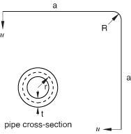
The pipeline configuration used in the study is shown in Figure 1. It is a simple model with two straight pipe sections connected by a 90° elbow. The straight pipes are 25.4 cm (10.0 inches) in length, the radius of the curved section is 10.16 cm (4.0 inches), and the outer radius of the pipe section is 1.27 cm (0.5 inches). The wall thickness of the pipe is varied from 0.03175 cm to 0.2032 cm (0.0125 inches to 0.08 inches) in a parametric study, as discussed below. The pipe material is assumed to be isotropic linear elastic with a Young's modulus of 194 GPa (28.1 × 10⁶ psi) and a Poisson's ratio of 0.0. The straight portions of the pipeline are assumed to be long enough so that warping at the ends of the structure is negligible.
Two loading conditions are analyzed. The first case is shown in Figure 1 with unit inward displacements imposed on both ends of the structure. This loading condition has the effect of closing the pipeline in on itself. In the second case the sense of the applied unit displacements is outward, opening the pipeline. Both cases are considered to be large-displacement/small-strain analyses.
A parametric study comparing the results obtained with different element types (shells, elbows, and pipes) over a range of flexibility factors, k, is performed. As defined in Dodge and Moore (1972), the flexibility factor for an elbow is the ratio of the bending flexibility of the elbow segment to that of a straight pipe of the same dimensions, assuming small displacements and an elastic response. When the internal (gauge) pressure is zero, as is assumed in this study, k can be approximated as
where
R is the bend radius of the curved section, r is the mean radius of the pipe, t is the wall thickness of the pipe, and is Poisson's ratio. Changes in the flexibility factor are introduced by varying the wall thickness of the pipe.
The pipeline is modeled with three different element types: S4 shell elements, ELBOW31 elbow elements, and PIPE31 pipe elements. The S4 shell element model consists of a relatively fine mesh of 40 elements about the circumference and 75 elements along the length. This mesh is deemed fine enough to capture the true response of the pipeline accurately, although no mesh convergence studies are performed. Two analyses are conducted with the shell mesh: one with automatic stabilization using a constant damping factor (see Automatic stabilization of static problems with a constant damping factor), and one with adaptive automatic stabilization (see Adaptive automatic stabilization scheme). The pipe and elbow element meshes consist of 75 elements along the length; the analyses with these element types do not use automatic stabilization.
The results of the shell element model with automatic stabilization using a constant damping factor are taken as the reference solution. The reaction force at the tip of the pipeline is used to evaluate the effectiveness of the pipe and elbow elements. In addition, the ovalization values of the pipeline cross-section predicted by the elbow element models are compared.
The elbow elements are tested with 0, 3, and 6 Fourier modes, respectively. In general, elbow element accuracy improves as more modes are used, although the computational cost increases accordingly. In addition to standard pipe elements, tests are performed on pipe elements with a special flexibility knockdown factor. Flexibility knockdown factors (Dodge and Moore, 1972) are corrections to the bending stiffness based upon linear semianalytical results. They are applied to simple beam elements in an attempt to capture the global effects of ovalization. The knockdown factor is implemented in the PIPE31 elements by scaling the true thickness by the flexibility factor; this is equivalent to scaling the moment of inertia of the pipe element by .
![]()
Results and discussion
The results obtained with the shell element model with automatic stabilization using a constant damping factor are taken as the reference solution. Very similar results are obtained with the same mesh using the adaptive automatic stabilization scheme.
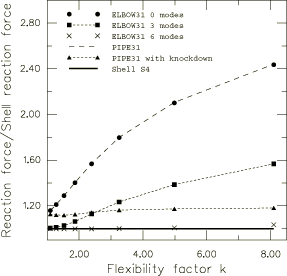
The tip reaction forces due to the inward prescribed displacements for the various analysis models are shown in Figure 2. The results are normalized with respect to those obtained with the shell model. The results obtained with the ELBOW31 element model with 6 Fourier modes show excellent agreement with the reference solution over the entire range of flexibility factors considered in this study. The remaining four models generally exhibit excessively stiff response for all values of k. The PIPE31 element model, which uses the flexibility knockdown factor, shows a relatively constant error of about 20% over the entire range of flexibility factors. The 0-mode ELBOW31 element model and the PIPE31 element model without the knockdown factor produce very similar results for all values of k.
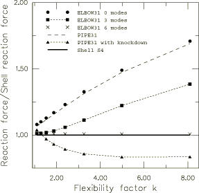
The normalized tip reaction forces due to the outward unit displacement for the various analysis models are shown in Figure 3. Again, the results obtained with the 6-mode ELBOW31 element model compare well with the reference shell solution. The 0-mode and 3-mode ELBOW31 and the PIPE31 (without the flexibility knockdown factor) element models exhibit overly stiff response. The PIPE31 element model with the knockdown factor has a transition region near k = 1.5, where the response changes from being too stiff to being too soft. The results in Abaqus/Explicit for pipe elements are consistent with those obtained in Abaqus/Standard.
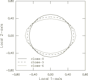
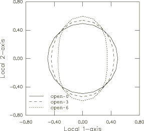
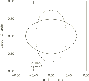
Figure 4 and Figure 5 illustrate the effect of the number of included Fourier modes (0, 3, and 6) on the ability of the elbow elements to model the ovalization in the pipebend accurately in both load cases considered in this study. By definition, the 0-mode model cannot ovalize, which accounts for its stiff response. The 3-mode and the 6-mode models show significant ovalization in both loading cases. Figure 6 compares the ovalization of the 6-mode model in the opened and closed deformation states. It clearly illustrates that when the ends of the pipe are displaced inward (closing mode), the height of the pipe's cross-section gets smaller, thereby reducing the overall stiffness of the pipe; the reverse is true when the pipe ends are displaced outward: the height of the pipe's cross-section gets larger, thereby increasing the pipe stiffness. These three figures were produced with the aid of the elbow element postprocessing program felbow.f (Creation of a data file to facilitate the postprocessing of elbow element results: FELBOW), written in Fortran. The postprocessing programs felbow.C (A C++ version of FELBOW) and felbow.py (An Abaqus Scripting Interface version of FELBOW), written in C++ and Python, respectively, are also available for generating the data for these figures. The user must ensure that the output variables are written to the output database to use these two programs.
![]()
Parametric study
The performance of the pipe and elbow elements investigated in this example is analyzed conveniently in a parametric study using the Python scripting capabilities of Abaqus (Scripting parametric studies). We perform a parametric study in which eight analyses are executed automatically for each of the three element types (S4, ELBOW31, and PIPE31) discussed above; these parametric studies correspond to wall thickness values ranging from 0.03175 cm to 0.2032 cm (0.0125 inches to 0.08 inches).
The Python script file elbowtest.psf is used to perform the parametric study. The function customTable (shown below) is an example of advanced Python scripting (Lutz and Ascher, 1999), which is used in elbowtest.psf. Such advanced scripting is not routinely needed, but in this case a dependent variable such as k cannot be included as a column of data in an XYPLOT file. customTable is designed to overcome this limitation by taking an XYPLOT file from the parametric study and converting it into a new file of reaction forces versus flexibility factors (k).
###############################################################
#
def customTable(file1, file2):
    for line in file1.readlines():
        print line
        nl = string.split(line,',')

        disp = float(nl[0])
        bend_radius = float(nl[1])
        wall_thick  = float(nl[2])
        outer_pipe_radius = float(nl[3])
        poisson = float(nl[4])
        rf = float(nl[6])

        mean_rad = outer_pipe_radius - wall_thick/2.0
        k = bend_radius*wall_thick/mean_rad**2
        k = k/sqrt(1.e0 - poisson**2)
        k = 1.66e0/k

        outputstring = str(k) + ', ' + str(rf) + '\n'
        file2.write(outputstring)
#
#############################################################
![]()
Input files
- elbowtest_shell.inp
-
S4 model.
- elbowtest_shell_stabil_adap.inp
-
S4 model with adaptive stabilization.
- elbowtest_elbow0.inp
-
ELBOW31 model with 0 Fourier modes.
- elbowtest_elbow3.inp
-
ELBOW31 model with 3 Fourier modes.
- elbowtest_elbow6.inp
-
ELBOW31 model with 6 Fourier modes.
- elbowtest_pipek.inp
-
PIPE31 model with the flexibility knockdown factor.
- elbowtest_pipek_xpl.inp
-
PIPE31 model with the flexibility knockdown factor in Abaqus/Explicit.
- elbowtest_pipe.inp
-
PIPE31 model without the flexibility knockdown factor.
- elbowtest_pipe_xpl.inp
-
PIPE31 model without the flexibility knockdown factor in Abaqus/Explicit.
- elbowtest.psf
-
Python script file for the parametric study.
![]()
References
- “Stress Indices and Flexibility Factors for Moment Loadings on Elbows and Curved Pipes,” Welding Research Council Bulletin, no. 179, 1972.
- Learning Python, O'Reilly, 1999.
![]()
Figures
