Contour integral evaluation: two-dimensional case | ||
| ||
ProductsAbaqus/Standard
The J-integral, stress intensity factors, and T-stress are widely used in fracture mechanics; and their accurate estimation for postulated flaws under given load conditions is an important aspect of the use of fracture mechanics in design. The domain integral method of Shih et al. (1986) provides a useful method for numerically evaluating contour integrals for the J-integral, stress intensity factors, and T-stress. This method provides high accuracy with rather coarse models in two dimensions; in three dimensions coarse meshes still give reasonably accurate values. It adds only a small increment to the cost of the stress analysis and can be specified easily. Abaqus offers the evaluation of these parameters for fracture mechanics studies based on either the conventional finite element method or the extended finite element method (XFEM). Contour integral evaluation is available in Abaqus for any loading (including thermal loading: see Single-edged notched specimen under a thermal load) and for elastic, elastic-plastic, and viscoplastic (creep) behaviors, the latter two cases being based on the equivalent hypoelastic material concept. The evaluation of the contour integral in three-dimensional cases is also often of interest: see Contour integral evaluation: three-dimensional case.
Problem description
Four examples are presented here for verification purposes. The first is a linear elastic, plane strain, double-edged notch specimen under Mode I loading, for which Bowie (1964) has provided a series solution for the stress intensity factor, ; the second is an axisymmetric specimen with a penny-shaped crack; the third is a single-edged notch specimen under Mode I loading; and the fourth is a bimaterial specimen with an interface crack lying along the interface between the two materials. For the plane strain case a three-dimensional model is also used, with one layer of elements in the thickness direction, to verify the capability for evaluating the J-integral as a function of position along the crack front. In this case the J-integral should be constant along the crack front—the same value as is obtained from the two-dimensional plane strain analysis. The submodeling technique is used to demonstrate how to obtain more accurate results around the crack tip. All four examples are studied based on the conventional finite element method. In addition, the first and the third examples are also studied based on the extended finite element method.
![]()
Geometry and model
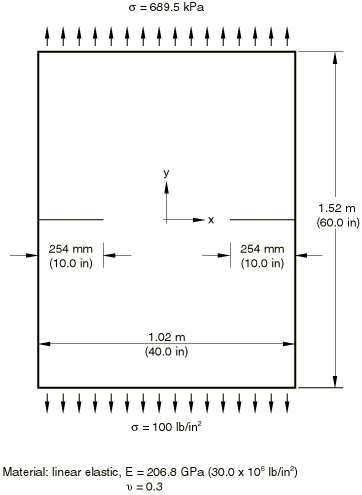
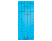
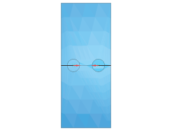
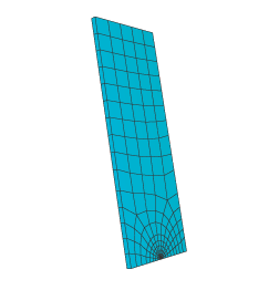
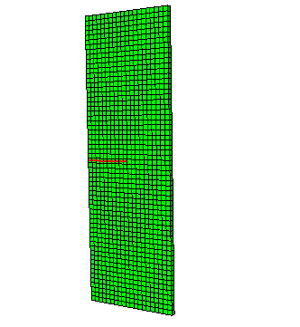
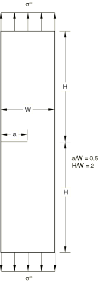
The geometry of the first example is shown in Figure 1. The plane strain structure is a section of a plate with symmetric edge cracks at its centerline, leaving an uncracked ligament of half the plate's width. The specimen is loaded in Mode I by uniform tension applied to its top and bottom surfaces. When the conventional finite element method is used, symmetry about x = 0 and about y = 0 can be used to model only the top right-hand quadrant of the plate. The mesh used for the quarter model is shown in Figure 2. Second-order elements (8-node quadrilaterals, 20-node bricks) are used. In the case of the full-model seam crack, left and right contour integrals are defined in Abaqus/CAE, as shown in Figure 3. Either the normal to the crack extension or the q vectors can be used to define the crack extension direction.
One advantage of using second-order elements with the conventional finite element method is that they can be used to model the desired singularity at the crack tip. To obtain a singularity term, the following conditions must be met:
The elements around the crack tip must be focused on the crack tip. One edge of each element must be collapsed to zero length (as shown in Figure 2) so that the nodes of this zero length edge are located at the crack tip.
The “midside” nodes of the edges radiating out from the crack tip of each of the elements attached to the crack tip must be placed at one-quarter of the distance from the crack tip to the other node of the edge.
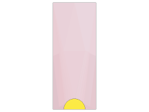
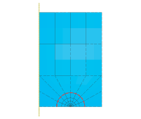
The region around the crack tip can be partitioned as shown in Figure 4 and swept meshed with elements having a quad-dominated shape. The node connectivity table is adjusted internally by Abaqus/CAE to create the degenerate quadrilateral elements.
If the coincident nodes at the crack tip are constrained to displace together, the only singularity term in strain is ; if the crack-tip nodes are free to displace independently, the crack-tip singularity in strain includes a term in addition to the term. These methods of creating singularities in standard isoparametric elements are explained in detail by Barsoum (1976).
The material type determines the singularity at the crack tip. A linear elastic material exhibits a singularity in strain at a sharp crack tip, whereas a perfectly plastic material exhibits a singularity in strain. The singularity in strain for a plastic hardening material lies somewhere between and .
Frequently the need for meshing simplicity with a preprocessor is greater than the need for extreme accuracy of contour integral results. The contour integral results often will be adequate as long as some singularity is included. For example, a singularity is introduced if the element edges are collapsed, the nodes at the crack tip are free to displace independently, and the midside nodes are not moved to the quarter points (they remain at the midside points). This singularity is often quite adequate for elastic-plastic problems.
The model in this example problem uses a linear elastic material and, thus, should be modeled with only a singularity term.
For the quarter model of the double-edged notch specimen, symmetry is used for calculating the contour integral results. Thus, the results for the contour integrals are multiplied by two before being output. The three-dimensional model uses the same mesh with one layer of 20-node bricks, as shown in Figure 5. The loading applied is either a uniform edge load in two dimensions or a uniform surface pressure (of negative magnitude) in three dimensions.
When the extended finite element method is used, the mesh is not required to match the cracked geometry. The presence of a crack is ensured by the special enriched functions in conjunction with additional degrees of freedom. This approach also removes the requirement to explicitly define the crack front or to specify the virtual crack extension direction when evaluating the contour integral. The data required for the contour integral will be determined automatically based on the level set signed distance functions at the nodes in an element. First-order brick elements with both full integration and reduced integration are used for this example. The mesh is shown in Figure 6.
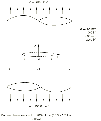
The axisymmetric model corresponds to a penny-shaped crack in a round bar. The model is shown in Figure 7 and is loaded in Mode I by uniform tension applied to the top and bottom surfaces. Symmetry about r = 0 and z = 0 allows you to model only the top right-hand quadrant with a mesh, as shown in Figure 8. Second-order elements (CAX8 and CAX8R) are used.
The third example is a single-edged notch specimen under Mode I tension, as shown in Figure 9. This specimen contains a crack in the symmetry plane in a homogeneous linear elastic material. This example has been studied using both the conventional finite element method and the extended finite element method. Due to symmetry only the top half-plane is modeled for the specimen when used with the conventional finite element method. The complete body is modeled when used with the extended finite element method. Second-order elements CPE8 and CPS8 are used with the conventional finite element method, while first-order brick elements C3D8 and first-order tetrahedral elements C3D4 are used with the extended finite element method.
The last example is also a single-edged notch specimen under Mode I tension, as shown in Figure 9. This specimen contains a crack lying along the interface between two dissimilar elastic materials. The complete body is modeled for the specimen with an interface crack. Second-order elements CPE8 and CPS8 are used for this example.
The J-integral, stress intensity factors, and T-stress should be path independent, and Abaqus provides for its evaluation on as many contours as you request. The first contour is normally at the crack tip, and subsequent contours are generated automatically as contours passing through the nearest neighboring elements, moving out from the crack tip. The mesh used in this case has several rings of elements surrounding the crack tip and as many contours as the number of rings that can be requested. The contour integral should be path independent, so the variation of values between contours can be taken as an indicator of the quality of the mesh for determining the fracture parameters. Path independence of the contour integral values is sufficient to indicate mesh convergence for stress, strain, or displacements.
![]()
Results and discussion
The plane strain solutions obtained with full- and reduced-integration elements (CPE8 and CPE8R) are compared with Bowie's approximate solution in Table 1 for the J-integral. The Abaqus results are very close to Bowie's approximation, and path independence is well preserved. The J-integral is also calculated automatically based on the stress intensity factors if the latter are requested by the contour integral evaluation of Abaqus. These J values show very good agreement with those presented in Table 1.
The three-dimensional solutions of the J-integral for the 20-node brick mesh are shown in Table 2. The J values provided by the fully integrated 20-node brick model show some oscillation along the crack front for the first contour. In the 20-node brick models contours involving midside nodes have fewer nodes being perturbed than contours involving corner nodes of such elements, which results in differences in strain energy calculations and, hence, in the integral values. The effect is not large and is generally apparent only for the first contour; it becomes smaller as the mesh is refined. Since the J values for this contour are also probably the least accurate regardless of the element type that is used, they are frequently ignored; and only the J values for contours two and higher are used in estimating J. The oscillation of the J-integral values with crack-front position is not evident in the reduced-integration models for the 20-node brick case. The stress intensity factors and the T-stress are also calculated for the same three-dimensional model. They have the same features as described above for the contour integral evaluation of J.
The three-dimensional solutions of the J-integral for the 8-node brick mesh using the extended finite element method are shown in Table 3.
The axisymmetric solutions of the J-integral are shown in Table 4, where they can be compared to an approximate solution from Tada et al. (1973). Path independence is well preserved in the mesh. The numerical results are again slightly higher than the approximate solution from Tada et al. (1973). However, the stress intensity factors and T-stress show evidence of contour dependence in this mesh. The crack tip is so close to the symmetry axis that the auxiliary plane strain crack-tip field cannot be used satisfactorily in the interaction method to extract their values. Using more concentrated, refined meshes around the crack tip eliminates the problem.
Both the stress intensity factor, , and the T-stress are calculated for the single-edged notch specimen. The results are compared with the values presented in Tada et al. (1973) in Table 5 and with the T-stress values presented in Nakamura and Parks (1991) in Table 6. The comparisons show good agreement. In addition, the results obtained using the extended finite element method at the midsurface of a three-dimensional single-edged notch specimen are presented in Table 7.
For the interface crack model, the calculated results for the stress intensity factors and J-integrals are presented in Table 8. It can be seen from Table 8 that, although the specimen is subjected to a pure Mode I loading, the value of is nonzero—a typical feature of an interfacial crack. Table 8 also indicates that J calculated from the stress intensity factors agrees very well with J calculated directly by Abaqus.
![]()
Submodeling around the crack tip
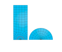
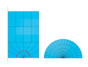
The submodeling technique is capable of providing a more accurate analysis of the stresses around the crack tip. The global model has a coarse mesh, while the submodel has a refined mesh. For the double-edged notch specimen and the single-edged notch specimen, the submodel region is a semicircular region of radius 127 mm (5 inches). Thus, the submodel boundary is the same as the partition around the crack tip in the global model. The submodel uses a focused mesh with six rows of elements around the crack tip. For the axisymmetric penny crack specimen, the submodel region is a semicircular region of radius 114.3 mm (4.5 inches) and coincides with the outer partition around the crack tip in the global model. The global mesh in all three problems gives satisfactory J-integral results; hence, we assume that the displacements at the submodel boundary are sufficiently accurate to drive the deformation in the submodel. No attempt has been made to study the effect of making the submodel region larger or smaller. The meshed global model with the boundary of the submodel (in dashed lines) is shown on the left, and on the right an enlarged view of the submodel is shown in Figure 10 and Figure 11 for the double-edged notch specimen and the axisymmetric penny crack specimen, respectively.
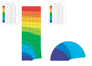
Contours of the vertical displacement field in the submodel and the global model are shown for a double-edged notch specimen in Figure 12. The continuity of the contour lines verifies that the proper displacement values are prescribed on the submodel boundary. Contour integral values are calculated using five contours. The results of the J-integral are listed in Table 9. The J-integral results obtained with the global mesh are quite accurate; hence, only minor improvements in J-integral values are expected. The same trend also prevails for the calculated stress intensity factor and the T-stress. The agreement with Bowie's approximate solution is indeed slightly better, and a somewhat better path independence can be observed as well. A submodel analysis is also carried out for the axisymmetric model. The calculated J-integral values for the submodel analysis of the axisymmetric penny crack are listed in Table 10.
![]()
Python scripts
- Full two-dimensional double-edged notch specimen meshed using fully integrated plane strain elements
Run the 2DDoubleEdgedNotchCPE8_model.py script to create the model. Then run the 2DDoubleEdgedNotchCPE8_job.py script to analyze the model.
- Full two-dimensional double-edged notch specimen meshed using reduced-integration plane strain elements
Run the 2DDoubleEdgedNotchCPE8R_model.py script to create the model. Then run the 2DDoubleEdgedNotchCPE8R_job.py script to analyze the model.
- Symmetric two-dimensional double-edged notch specimen meshed using fully integrated plane strain elements
Run the 2DDoubleEdSymmCPE8_model.py script to create the model. Then run the 2DDoubleEdSymmCPE8_job.py script to analyze the model.
- Symmetric two-dimensional double-edged notch specimen meshed using reduced-integration plane strain elements
Run the 2DDoubleEdSymmCPE8R_model.py script to create the model. Then run the 2DDoubleEdSymmCPE8R_job.py script to analyze the model.
- Submodel analysis of a symmetric two-dimensional double-edged notch specimen meshed using fully integrated plane strain elements
The analysis is done in two stages:
Run the 2DDoubleEdSymmGlCPE8_model.py script to create the global model. Then run the 2DDoubleEdSymmGlCPE8_job.py script to analyze the global model and to create the output database (.odb) file that will drive the submodel.
Run the 2DDoubleEdSymmSubCPE8_model.py script to create the submodel. Then run the 2DDoubleEdSymmSubCPE8_job.py script to analyze the submodel using the output database file from the global model to drive it.
- Submodel analysis of a symmetric two-dimensional double-edged notch specimen meshed using reduced-integration plane strain elements
The analysis is done in two stages:
Run the 2DDoubleEdSymmGlCPE8R_model.py script to create the global model. Then run the 2DDoubleEdSymmGlCPE8R_job.py script to analyze the global model and to create the output database (.odb) file that will drive the submodel.
Run the 2DDoubleEdSymmSubCPE8R_model.py script to create the submodel. Then run the 2DDoubleEdSymmSubCPE8R_job.py script to analyze the submodel using the output database file from the global model to drive it.
- Symmetric two-dimensional single-edged notch specimen meshed using fully integrated plane strain elements
Run the 2DSingleEdgedSymmCPE8_model.py script to create the model. Then run the 2DSingleEdgedSymmCPE8_job.py script to analyze the model.
- Symmetric two-dimensional single-edged notch specimen meshed using fully integrated plane stress elements
Run the 2DSingleEdgedSymmCPS8_model.py script to create the model. Then run the 2DSingleEdgedSymmCPS8_job.py script to analyze the model.
- Submodel analysis of a symmetric two-dimensional single-edged notch specimen meshed using fully integrated plane strain elements
The analysis is done in two stages:
Run the 2DSingleEdSymmGlCPE8_model.py script to create the global model. Then run the 2DSingleEdSymmGlCPE8_job.py script to analyze the global model and to create the output database (.odb) file that will drive the submodel.
Run the 2DSingleEdSymmSubCPE8_model.py script to create the submodel. Then run the 2DSingleEdSymmSubCPE8_job.py script to analyze the submodel using the output database file from the global model to drive it.
- Submodel analysis of a symmetric two-dimensional single-edged notch specimen meshed using fully integrated plane stress elements
The analysis is done in two stages:
Run the 2DSingleEdSymmGlCPS8_model.py script to create the global model. Then run the 2DSingleEdSymmGlCPS8_job.py script to analyze the global model and to create the output database (.odb) file that will drive the submodel.
Run the 2DSingleEdSymmSubCPS8_model.py script to create the submodel. Then run the 2DSingleEdSymmSubCPS8_job.py script to analyze the submodel using the output database file from the global model to drive it.
- Axisymmetric penny-shaped crack specimen meshed using fully integrated axisymmetric elements
Run the 2DAxPennyCrackCAX8_model.py script to create the model. Then run the 2DAxPennyCrackCAX8_job.py script to analyze the model.
- Axisymmetric penny-shaped crack specimen meshed using reduced-integration axisymmetric elements
Run the 2DAxPennyCrackCAX8R_model.py script to create the model. Then run the 2DAxPennyCrackCAX8R_job.py script to analyze the model.
- Submodel analysis of an axisymmetric penny-shaped crack specimen meshed using fully integrated axisymmetric elements
The analysis is done in two stages:
Run the 2DAxPennyCrackGlCAX8_model.py script to create the global model. Then run the 2DAxPennyCrackGlCAX8_job.py script to analyze the global model and to create the output database (.odb) file that will drive the submodel.
Run the 2DAxPennyCrackSubCAX8_model.py script to create the submodel. Then run the 2DAxPennyCrackSubCAX8_job.py script to analyze the submodel using the output database file from the global model to drive it.
- Submodel analysis of an axisymmetric penny-shaped crack specimen meshed using reduced-integration axisymmetric elements
The analysis is done in two stages:
Run the 2DAxPennyCrackGlCAX8R_model.py script to create the global model. Then run the 2DAxPennyCrackGlCAX8R_job.py script to analyze the global model and to create the output database (.odb) file that will drive the submodel.
Run the 2DAxPennyCrackSubCAX8R_model.py script to create the submodel. Then run the 2DAxPennyCrackSubCAX8R_job.py script to analyze the submodel using the output database file from the global model to drive it.
- Symmetric three-dimensional double-edged notch specimen meshed using fully integrated plane continuum elements
Run the 3DDoubleEdgedNotchC3D20_model.py script to create the model. Then run the 3DDoubleEdgedNotchC3D20_job.py script to analyze the model.
- Symmetric three-dimensional double-edged notch specimen meshed using reduced-integration continuum elements
Run the 3DDoubleEdgedNotchC3D20R_model.py script to create the model. Then run the 3DDoubleEdgedNotchC3D20R_job.py script to analyze the model.
- Symmetric two-dimensional plane strain single-edged notch specimen containing an interface crack
Run the 2DDissimilarMaterialsCPE8_model.py script to create the model. Then run the 2DDissimilarMaterialsCPE8_job.py script to analyze the model.
![]()
Input files
The input files listed below are provided for users who prefer to use the Abaqus keyword interface instead of Abaqus/CAE. The meshes created in these input files are different from those created by using the Python scripts; however, the results are of the same accuracy.
- jintegral2d_cpe8.inp
Two-dimensional plane strain model with full integration.
- jintegral2d_cpe8r.inp
Two-dimensional plane strain model with reduced integration.
- jintegral2d_cpe4_residual.inp
Two-dimensional first-order plane strain model with full integration and the effect of a residual stress field.
- jintegral2d_cpe8_submodel.inp
Two-dimensional plane strain submodel with full integration.
- jintegral2d_c3d20.inp
20-node brick three-dimensional model with full integration.
- jintegral2d_postoutput.inp
POST OUTPUT analysis of jintegral2d_c3d20.inp.
- jintegral2d_c3d20r.inp
20-node brick three-dimensional model with reduced integration.
- jintegral2d_c3d27.inp
27-node brick three-dimensional model with full integration.
- jintegral2d_c3d27r.inp
27-node brick three-dimensional model with reduced integration.
- jintegral2d_cax8.inp
Axisymmetric model with full integration.
- jintegral2d_cax8r.inp
Axisymmetric model with reduced integration.
- jintegral2d_cax8_submodel.inp
Axisymmetric submodel with full integration.
- jintegral2d_3daxi.inp
20-node brick three-dimensional model of the axisymmetric problem with reduced integration.
- cintegral2d_1edge_cpe8.inp
Two-dimensional plane strain model for single-edged notch specimen.
- cintegral2d_1edge_cps8.inp
Two-dimensional plane stress model for single-edged notch specimen.
- cintegral2d_1edge_intf_cpe8.inp
Two-dimensional plane strain model for single-edged notch specimen containing an interface crack.
- contourintegral_den_xfem_c3d8.inp
8-node brick three-dimensional model with full integration for double-edged notch specimen with extended finite element method.
- contourintegral_den_xfem_c3d8r.inp
8-node brick three-dimensional model with reduced integration for double-edged notch specimen with extended finite element method.
- contourintegral_sen_xfem_c3d8.inp
8-node brick three-dimensional model with full integration for single-edged notch specimen with extended finite element method.
- contourintegral_sen_xfem_c3d8_base.inp
Same as contourintegral_sen_xfem_c3d8.inp but including the plasticity to generate a residual stress field.
- contourintegral_sen_xfem_c3d8_residual.inp
Same as contourintegral_sen_xfem_c3d8.inp but including the effect of a residual stress field that was generated from the analysis of contourintegral_sen_xfem_c3d8_base.
- contourintegral_sen_xfem_c3d4.inp
4-node tetrahedron three-dimensional model for single-edged notch specimen with extended finite element method.
![]()
References
- “On the Use of Isoparametric Finite Elements in Linear Fracture Mechanics,” International Journal for Numerical Methods in Engineering, vol. 10, pp. 25–37, 1976.
- “Rectangular Tensile Sheet With Symmetric Edge Cracks,” Journal of Applied Mechanics, vol. 31, pp. 208–212, 1964.
- “Determination of Elastic T-Stress along Three-Dimensional Crack Fronts Using an Interaction Integral,” International Journal of Solids and Structures, vol. 28, pp. 1597–1611, 1991.
- “Energy Release Rate along a Three-Dimensional Crack Front in a Thermally Stressed Body,” International Journal of Fracture, vol. 30, pp. 79–102, 1986.
- The Stress Analysis of Cracks Handbook, Del Research Corporation, Hellertown, Pennsylvania, 1973.
![]()
Tables
| Contour | Full integration | Reduced integration | ||
|---|---|---|---|---|
| N/m | lb/in | N/m | lb/in | |
| 1 | 2.284 | 0.01303 | 2.285 | 0.01304 |
| 2 | 2.282 | 0.01302 | 2.280 | 0.01301 |
| 3 | 2.282 | 0.01302 | 2.282 | 0.01302 |
| 4 | 2.282 | 0.01302 | 2.282 | 0.01302 |
| 5 | 2.282 | 0.01302 | 2.282 | 0.01302 |
| Full integration | ||||||
| Contour | Front face | Middle surface | Back face | |||
| N/m | lb/in | N/m | lb/in | N/m | lb/in | |
| 1 | 2.212 | 0.01262 | 2.306 | 0.01316 | 2.212 | 0.01262 |
| 2 | 2.277 | 0.01299 | 2.277 | 0.01299 | 2.277 | 0.01299 |
| 3 | 2.280 | 0.01301 | 2.280 | 0.01301 | 2.280 | 0.01301 |
| Reduced integration | ||||||
| Contour | Front face | Middle surface | Back face | |||
| N/m | lb/in | N/m | lb/in | N/m | lb/in | |
| 1 | 2.273 | 0.01297 | 2.284 | 0.01303 | 2.273 | 0.01297 |
| 2 | 2.277 | 0.01299 | 2.277 | 0.01299 | 2.277 | 0.01299 |
| 3 | 2.280 | 0.01301 | 2.280 | 0.01301 | 2.280 | 0.01301 |
| Full integration | ||||
| Contour | Front face | Back face | ||
| N/m | lb/in | N/m | lb/in | |
| 3 | 2.874 | 0.01641 | 2.874 | 0.01641 |
| 4 | 2.795 | 0.01596 | 2.795 | 0.01596 |
| 5 | 3.108 | 0.01775 | 3.108 | 0.01775 |
| 6 | 2.559 | 0.01461 | 2.559 | 0.01461 |
| 7 | 2.343 | 0.01338 | 2.343 | 0.01338 |
| 8 | 2.485 | 0.01419 | 2.485 | 0.01419 |
| Reduced integration | ||||
| Contour | Front face | Back face | ||
| N/m | lb/in | N/m | lb/in | |
| 3 | 2.884 | 0.01647 | 2.884 | 0.01647 |
| 4 | 2.799 | 0.01598 | 2.799 | 0.01598 |
| 5 | 3.112 | 0.01777 | 3.112 | 0.01777 |
| 6 | 2.567 | 0.01466 | 2.567 | 0.01466 |
| 7 | 2.361 | 0.01348 | 2.361 | 0.01348 |
| 8 | 2.494 | 0.01424 | 2.494 | 0.01424 |
| Contour | Full integration | Reduced integration | ||
|---|---|---|---|---|
| N/m | lb/in | N/m | lb/in | |
| 1 | 0.7870 | 0.00449 | 0.7853 | 0.00448 |
| 2 | 0.7818 | 0.00446 | 0.7853 | 0.00448 |
| 3 | 0.7835 | 0.00447 | 0.7870 | 0.00449 |
| 4 | 0.7835 | 0.00447 | 0.7870 | 0.00449 |
| 5 | 0.7835 | 0.00447 | 0.7870 | 0.00449 |
| Contour | CPE8 | CPS8 |
|---|---|---|
| 1 | 2.8250 | 2.8249 |
| 2 | 2.8230 | 2.8231 |
| 3 | 2.8237 | 2.8238 |
| 4 | 2.8238 | 2.8239 |
| 5 | 2.8238 | 2.8239 |
| Contour | CPE8 | CPS8 |
|---|---|---|
| 1 | –0.4307 | –0.4298 |
| 2 | –0.4204 | –0.4202 |
| 3 | –0.4226 | –0.4224 |
| 4 | –0.4226 | –0.4224 |
| 5 | –0.4225 | –0.4223 |
| Contour | C3D8 | C3D4 |
|---|---|---|
| 2 | 2.8537 | 2.8871 |
| 3 | 2.9643 | 2.8675 |
| 4 | 3.0027 | 2.8675 |
| 5 | 2.9696 | 2.9014 |
| Contour | J-integral value estimated by the stress intensity factors | J-integral value estimated directly | ||
|---|---|---|---|---|
| from | ||||
| 1 | 2.8245 | 0.0121 | 17.36 | 17.30 |
| 2 | 2.8226 | 0.0127 | 17.33 | 17.30 |
| 3 | 2.8232 | 0.0127 | 17.34 | 17.30 |
| 4 | 2.8233 | 0.0127 | 17.34 | 17.30 |
| 5 | 2.8232 | 0.0127 | 17.34 | 17.30 |
| Contour | Full integration | Reduced integration | ||
|---|---|---|---|---|
| N/m | lb/in | N/m | lb/in | |
| 1 | 2.282 | 0.01302 | 2.285 | 0.01304 |
| 2 | 2.278 | 0.013 | 2.280 | 0.01301 |
| 3 | 2.280 | 0.01301 | 2.282 | 0.01302 |
| 4 | 2.280 | 0.01301 | 2.282 | 0.01302 |
| 5 | 2.280 | 0.01301 | 2.282 | 0.01302 |
| Contour | Full integration | Reduced integration | ||
|---|---|---|---|---|
| N/m | lb/in | N/m | lb/in | |
| 1 | 0.7765 | 0.00443 | 0.7853 | 0.00448 |
| 2 | 0.7748 | 0.00442 | 0.7835 | 0.00447 |
| 3 | 0.7765 | 0.00443 | 0.7835 | 0.00447 |
| 4 | 0.7765 | 0.00443 | 0.7835 | 0.00447 |
| 5 | 0.7765 | 0.00443 | 0.7835 | 0.00447 |
![]()
Figures
