Generate a history plot of the axial stress in the pipe for the restart
analysis
In the
Results Tree,
double-click XYData.
The Create XY Data dialog box appears.
Select ODB field output from this dialog box, and
click Continue to proceed.
The XY Data from ODB Field Output dialog box
appears.
In the Variables tabbed page of this dialog box,
accept the default selection of Integration
Point for the variable position and select
S11 from the list of available stress components.
At the bottom of the dialog box, toggle Select
for the section point and click Settings to choose a
section point.
In the Field Report Section Point Settings dialog
box that appears, select the category beam and
choose any of the available section points for the pipe cross-section. Click
OK to exit this dialog box.
In the Elements/Nodes tabbed page of the
XY Data from ODB Field Output dialog box, select
Element labels as the selection
Method. There are 30 elements in the model, and they are
numbered consecutively from 1 to 30. Enter any element number (for example,
25) in the Element labels
text field that appears on the right side of the dialog box.
Click Active Steps/Frames, and select
Pull II as the only step from which to
extract data.
At the bottom of the XY Data from ODB Field
Output dialog box, click Plot to see the
history of axial stress in the element.
The plot traces the axial stress history at each integration point of
the element in the restart analysis. Since the restart is a continuation of an
earlier job, it is often useful to view the results from the entire (original
and restarted) analysis.

Generate a history plot of the axial stress in the pipe for the entire
analysis
Save the current plot by clicking Save at the
bottom of the XY Data from ODB Field Output dialog box.
Two curves are saved (one for each integration point), and default names are
given to the curves.
Rename either curve RESTART, and delete
the other curve.
From the main menu bar, select
;
or use the
 tool in the
File toolbar
to open the file Pipe.odb. tool in the
File toolbar
to open the file Pipe.odb.
Following the procedure outlined above, save the plot of the axial
stress history for the same element and integration/section point used above.
Name this plot ORIGINAL.
In the
Results Tree,
expand the XYData container.
The ORIGINAL and
RESTART curves are listed underneath.
Select both plots with
CtrlClick.
Click mouse button 3, and select Plot from the menu that
appears to create a plot of axial stress history in the pipe for the entire
simulation.
To change the style of the line, open the Curve
Options dialog box.
For the RESTART curve, select a dotted
line style.
Click Dismiss to close the dialog box.
To change the axis titles, open the Axis Options
dialog box.
In this dialog box, switch to the Title tabbed
page.
Change the X-axis title to
TOTAL TIME, and change the
Y-axis title to STRESS
S11.
Click Dismiss to close the dialog box.
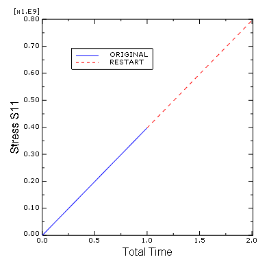
The plot created by these commands is shown in
Figure 1.
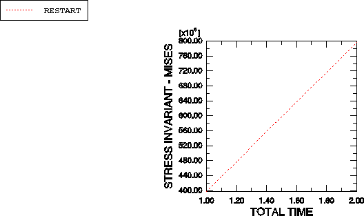
The axial stress history of the same element during Step 3 can be plotted by
itself by selecting only the RESTART curve (see
Figure 2).
Figure 1. History of axial stress in the pipe.

Figure 2. History of axial stress in the pipe during Step 3.

|
![]()