Discussion of the two forming attempts | ||
| ||
The additional requirements—that the histories of kinetic energy and internal energy must be appropriate and reasonable—are very useful and necessary, but they also increase the subjectivity of evaluating the results. Enforcing these requirements in general for more complex forming processes may be difficult because these requirements demand some intuition regarding the behavior of the forming process.
- Results of the forming analysis
-
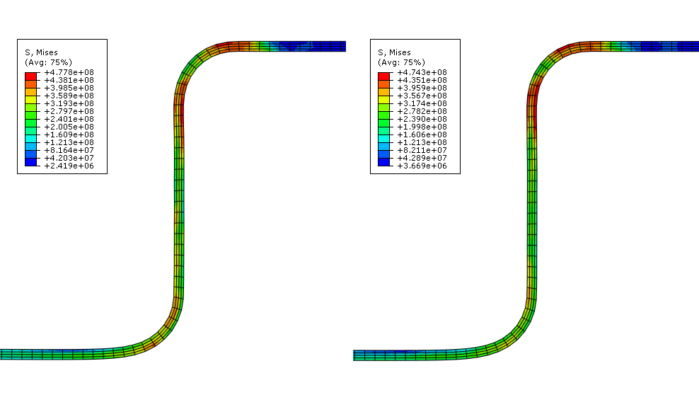
Now that we are satisfied that the quasi-static solution for the forming analysis is adequate, we can study some of the other results of interest. Figure 1 shows a comparison of the Mises stress in the blank obtained with Abaqus/Standard and Abaqus/Explicit.
Figure 1. Contour plot of Mises stress in Abaqus/Standard (left) and Abaqus/Explicit (right) channel forming analyses.
The plot shows that the peak stresses in the Abaqus/Standard and Abaqus/Explicit analyses are within 1% of each other and that the overall stress contours of the blank are very similar. To further examine the validity of the quasi-static analysis results, you should compare the equivalent plastic strain results and final deformed shapes from the two analyses.
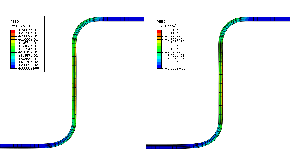
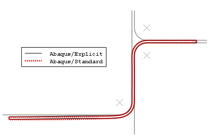
Figure 2 shows contour plots of the equivalent plastic strain in the blank, and Figure 3 shows an overlay plot of the final deformed shape predicted by the two analyses.
Figure 2. Contour plot of PEEQ in Abaqus/Standard (left) and Abaqus/Explicit (right) channel forming analyses.
Figure 3. Final deformed shape in Abaqus/Standard and Abaqus/Explicit forming analyses.
The equivalent plastic strain results for the Abaqus/Standard and Abaqus/Explicit analyses are within 5% of each other. In addition, the final deformed shape comparison shows that the explicit quasi-static analysis results are in excellent agreement with the results from the Abaqus/Standard static analysis.
You should also compare the steady punch force predicted by the Abaqus/Standard and Abaqus/Explicit analyses.
To compare the punch force-displacement histories:
-
Save the punch displacement (U2) and reaction force (RF2) history data from the Abaqus/Standard analysis as U2–std and RF2–std, respectively.
-
Similarly, save punch displacement (U2) and reaction force (RF2) history data from the Abaqus/Explicit analysis as U2–xpl and RF2–xpl, respectively.
Next, you will operate on saved X–Y data to create the force-displacement curves. In the force-displacement plot we would like the downward motion of the punch to be represented as a positive value; therefore, when you create the force-displacement curves include a negative sign before the displacement history data so that motion in the negative 2-direction will be positive.
-
In the Results Tree, double-click XYData; then select in the Create XY Data dialog box. Click .
-
In the Operate on XY Data dialog box, combine the force and displacement history data from the Abaqus/Standard analysis to create a force-displacement curve. The expression at the top of the dialog box should appear as:
combine ( -"U2-std", "RF2-std" )
-
Click to save the calculated displacement curve as forceDisp-std.
-
In the Operate on XY Data dialog box, combine the force and displacement history data from the Abaqus/Explicit analysis to create a force-displacement curve. The expression at the top of the dialog box should appear as:
combine ( -"U2-xpl", "RF2-xpl" )
-
Click to save the calculated displacement curve as forceDisp-xpl.
-
Plot forceDisp-std and forceDisp-xpl in the viewport.
There is significantly more noise in the Abaqus/Explicit results compared to the Abaqus/Standard results because Abaqus/Explicit simulates a quasi-static response while Abaqus/Standard solves for true static equilibrium. Some of the noise in the Abaqus/Explicit history data was removed during the analysis by the built-in antialiasing filter specified on the output request. Now, you will use an Abaqus/CAE X–Y data filter to remove more of the solution noise from the Abaqus/Explicit force-displacement curve. The Abaqus/CAE X–Y data filters should only be applied to X–Y data whose X-value is time. This avoids confusion regarding the meaning of the filter cutoff frequency and prevents problems with the data regularization that is performed internally before the filter is applied. Consequently, you will not filter forceDisp-xpl directly, but rather you will filter U2-xpl and RF2-xpl individually before combining them to create a new force-displacement curve. It is best to apply the same filter operations (both during the analysis and during postprocessing) to any two X–Y data objects that will be combined. This will ensure that any distortions due to filtering (such as time delays) are uniformly applied to the combined data.
-
In the Operate on XY Data dialog box, filter the force history data using a Butterworth filter with a cutoff frequency of 1100 Hz. The expression at the top of the dialog box should appear as:
butterworthFilter(xyData="RF2-xpl",cutoffFrequency=1100)
Note:
Choosing an appropriate filter cutoff frequency takes engineering judgment and a good understanding of the physical system being modeled. Often an iterative approach (beginning with a relatively high cutoff frequency and then gradually reducing it) can be used to find a cutoff frequency that removes solution noise with minimal distortion of the underlying physical solution. Knowledge of the system's natural frequencies can also assist in the determination of appropriate filter cutoff frequencies. For this example, we performed a frequency extraction analysis to determine the fundamental frequency of the undeformed blank (140 Hz); however, the blank at the end of the forming step will have a fundamental frequency that is considerably higher. If you perform a natural frequency extraction analysis on the final model configuration, you will find that the fundamental frequency at the end of the forming step is approximately 1000 Hz. Hence, a cutoff frequency that is slightly larger than this value is a good choice for this model.
-
Click to save the calculated displacement curve as RF2-xpl-bw1100.
-
Similarly, filter the displacement history data using a Butterworth filter with a cutoff frequency of 1100 Hz. The expression at the top of the Operate on XY Data dialog box should appear as:
butterworthFilter(xyData="U2-xpl",cutoffFrequency=1100)
-
Click to save the calculated displacement curve as U2-xpl-bw1100.
-
Combine the filtered Abaqus/Explicit force and displacement histories. The expression at the top of the Operate on XY Data dialog box should appear as:
combine ( -"U2-xpl-bw1100", "RF2-xpl-bw1100" )
-
Click to save the calculated displacement curve as forceDisp-xpl-bw1100.
-
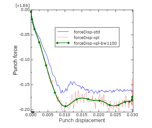
Add forceDisp-xpl-bw1100 to the plot of forceDisp-std and forceDisp-xpl. Customize the plot appearance to obtain a plot similar to Figure 4.
Figure 4. Steady punch force comparison for Abaqus/Standard and Abaqus/Explicit.
As seen in Figure 4, the steady punch force predicted by Abaqus/Explicit is approximately 12% higher than that predicted by Abaqus/Standard. The differences between the Abaqus/Standard and Abaqus/Explicit results are primarily due to two factors. First, Abaqus/Explicit regularizes the material data. Second, friction effects are handled slightly differently in the two analysis products; Abaqus/Standard uses penalty friction, whereas Abaqus/Explicit uses kinematic friction.
-
From these comparisons it is clear that both Abaqus/Standard and Abaqus/Explicit are capable of handling difficult contact analyses such as this one. However, there are some advantages to running this type of analysis in Abaqus/Explicit: Abaqus/Explicit is able to handle complex contact conditions more readily. However, when choosing Abaqus/Explicit for quasi-static analysis, you should be aware that you may need to iterate on an appropriate loading rate. In determining the loading rate, it is recommended that you begin with faster loading rates and decrease the loading rate as necessary. This will help optimize the run time for the analysis.