Postprocessing the results | ||
| ||
- Deformed model shape and peak displacements
-
Plot the deformed model shape with these new results, and change the deformation scale factor to 2 to obtain a plot similar to Figure 1. The displayed deformations are double the actual deformations.
Figure 1. Deformed model shape for the simulation with plastic hardening.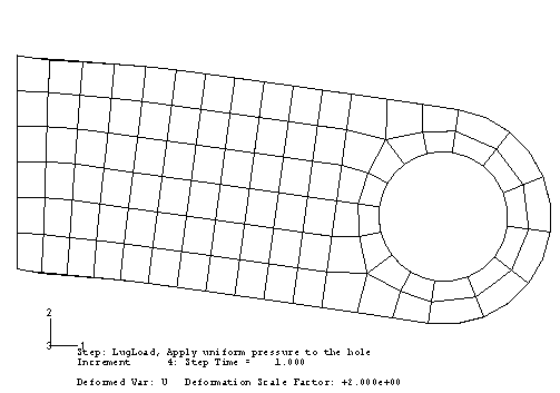
- Contour plot of Mises stress
-
Contour the Mises stress in the model. Create a filled contour plot using ten contour intervals on the actual deformed shape of the lug (i.e., set the deformation scale factor to 1.0) with the plot title and state blocks suppressed. Use the view manipulation tools to position and size the model to obtain a plot similar to that shown in Figure 2.
Figure 2. Contour of Mises stress.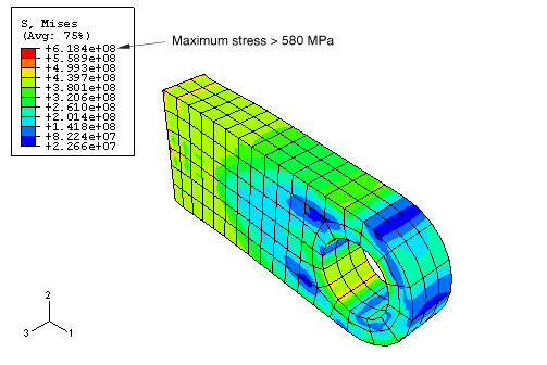
Do the values listed in the contour legend surprise you? The maximum stress is greater than 580 MPa, which should not be possible since the material was assumed to be perfectly plastic at this stress magnitude. This misleading result occurs because of the algorithm that Abaqus/CAE uses to create contour plots for element variables, such as stress. The contouring algorithm requires data at the nodes; however, Abaqus/Standard calculates element variables at the integration points. Abaqus/CAE calculates nodal values of element variables by extrapolating the data from the integration points to the nodes. The extrapolation order depends on the element type; for second-order, reduced-integration elements Abaqus/CAE uses linear extrapolation to calculate the nodal values of element variables. To display a contour plot of Mises stress, Abaqus/CAE extrapolates the stress components from the integration points to the nodal locations within each element and calculates the Mises stress. If the differences in Mises stress values fall within the specified averaging threshold, nodal averaged Mises stresses are calculated from each surrounding element's invariant stress value. Invariant values exceeding the elastic limit can be produced by the extrapolation process.
Try plotting contours of each component of the stress tensor (variables S11, S22, S33, S12, S23, and S13). You will see that there are significant variations in these stresses across the elements at the built-in end. This causes the extrapolated nodal stresses to be higher than the values at the integration points. The Mises stress calculated from these values will, therefore, also be higher.
Note:
Surface integration elements (C3D8S, C3D8HS, and C3D10HS) do not suffer from this extrapolation problem. The integration points of these element types are located at the nodes, resulting in improved surface stress visualization.
The Mises stress at an integration point can never exceed the current yield stress of the element's material; however, the extrapolated nodal values reported in a contour plot may do so. In addition, the individual stress components may have magnitudes that exceed the value of the current yield stress; only the Mises stress is required to have a magnitude less than or equal to the value of the current yield stress.
You can use the query tools in the Visualization module to check the Mises stress at the integration points.
To query the Mises stress:
-
From the main menu bar, select ; or use the
 tool in the
Query toolbar.
The Query dialog box appears.
-
In the Visualization Module Queries field, select Probe values.
The Probe Values dialog box appears.
-
Make sure that Elements and the output position Integration Pt are selected.
-
Use the cursor to select elements near the constrained end of the lug.
Abaqus/CAE reports the element ID and type by default and the value of the Mises stress at each integration point starting with the first integration point. The Mises stress values at the integration points are all lower than the values reported in the contour legend and also below the yield stress of 580 MPa. You can click mouse button 1 to store probed values.
-
Click when you have finished probing the results.
The fact that the extrapolated values are so different from the integration point values indicates that there is a rapid variation of stress across the elements and that the mesh is too coarse for accurate stress calculations. This extrapolation error will be less significant if the mesh is refined but will always be present to some extent. Therefore, always use nodal values of element variables with caution.
-
- Contour plot of equivalent plastic strain
-
The equivalent plastic strain in a material (PEEQ) is a scalar variable that is used to represent the material's inelastic deformation. If this variable is greater than zero, the material has yielded. Those parts of the lug that have yielded can be identified in a contour plot of PEEQ by selecting Primary from the list of variable types on the left side of the Field Output toolbar and selecting PEEQ from the list of output variables. Any areas in the model plotted in a dark color in Abaqus/CAE still have elastic material behavior (see Figure 3).
Figure 3. Contour of equivalent plastic strain (PEEQ).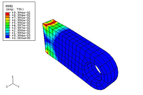
It is clear from the plot that there is gross yielding in the lug where it is attached to its parent structure. The maximum plastic strain reported in the contour legend is about 10%. However, this value may contain errors from the extrapolation process. Use the query tool
 to check the integration point values of PEEQ in the elements with the largest plastic strains. You will find
that the largest equivalent plastic strains in the model are about 0.087 at the
integration points. This does not necessarily indicate a large extrapolation
error since there are strain gradients present in the vicinity of the peak
plastic deformation.
- Creating a variable-variable (stress-strain) plot
-
The X–Y plotting capability in Abaqus/CAE was introduced earlier in this guide. In this section you will learn how to create X–Y plots showing the variation of one variable as a function of another. You will use the stress and strain data saved to the output database (.odb) file (in the form of field output rather than history output) to create a stress-strain plot for one of the integration points in an element adjacent to the constrained end of the lug.
Consider the shaded element shown in Figure 4.
Figure 4. Element where stress and strain histories will be studied.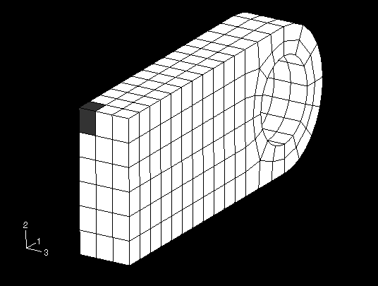
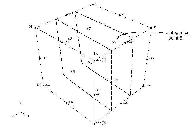
We will plot the stress and strain histories at an integration point in this element. The selected integration point should be as close as possible to the top surface of the lug but not adjacent to the constrained nodes. The numbering of the integration points depends on the element's nodal connectivity. Thus, you will need to identify the element's label as well as its nodal connectivity to determine which integration point to use.
To determine the integration point number:
-
In the Display Group toolbar, select the Replace Selected
 tool and click the shaded element shown in
Figure 4.
-
Plot the undeformed shape of this element with the node labels made visible. Click the auto-fit tool
 to obtain a plot similar to
Figure 5.
Figure 5. Location of integration point near the top surface.
-
Use the Query tool to obtain the nodal connectivity for this corner element (select Element, and click the element in the viewport). The nodal connectivity will be printed to the message area; you are interested in only the first four nodes.
-
Compare the nodal connectivity list with the undeformed model shape plot to determine which is the 1–2–3–4 face on your C3D20R element, as defined in Three-dimensional solid element library. For example, in Figure 5 the 276–552–313–79 face corresponds to the 1–2–3–4 face. Thus, the integration points are numbered as shown in the figure. We are interested in the point that corresponds to integration point 5.
In the following discussion, assume that the element label is 41 and that integration point 5 of this element satisfies the requirements stated above. Your element and/or integration point numbers may differ.
To create history curves of stress and direct strain along the
lug:
-
In the Results Tree, double-click XYData.
The Create XY Data dialog box appears.
-
In this dialog box, select ODB field output as the source and click Continue.
The XY Data from ODB Field Output dialog box appears; the Variables tabbed page is open by default.
-
In this dialog box, expand the following lists: S: Stress components and E: Strain components.
-
From the list of available stress and strain components, select Mises and E11, respectively.
The Mises stress, rather than the component of the true stress tensor, is used because the plasticity model defines plastic yield in terms of Mises stress. The E11 strain component is used because it is the largest component of the total strain tensor at this point; using it clearly shows the elastic, as well as the plastic, behavior of the material at this integration point.
-
Click the Elements/Nodes tab.
-
Accept Pick from viewport as the selection method, and click Edit Selection.
-
In the viewport, click the shaded element shown in Figure 4, then click Done in the prompt area.
-
Click Save to save the data followed by to close the dialog box.
Sixteen curves are created (one for each variable at each integration point), and default names are given to the curves. The curves appear in the XYData container. Each of the curves is a history (variable versus time) plot. You must combine the plots for the integration point of interest, eliminating the time dependence, to produce the desired stress-strain plot.
To combine history curves to produce a stress-strain
plot:
-
In the Results Tree, double-click XYData.
The Create XY Data dialog box appears.
-
Select Operate on XY data, and click .
The Operate on XY Data dialog box appears. Expand the Name field to see the full name of each curve.
-
From the Operators listed, select .
combine( ) appears in the text field at the top of the dialog box.
-
In the XY Data field, select the stress and strain curves for the integration point of interest.
-
Click . The expression combine("E:E11 ...", "S:MISES ...") appears in the text field. In this expression "E:E11 ..." will determine the X-values and "S:MISES ..." will determine the Y-values in the combined plot.
-
Save the combined data object by clicking at the bottom of the dialog box.
The Save XY Data As dialog box appears. In the Name text field, type SVE11; and click to close the dialog box.
-
To view the combined stress-strain plot, click at the bottom of the dialog box.
-
Click to close the dialog box.
-
Click
 in the prompt area to cancel the current procedure.
This X–Y plot would be clearer if the limits on the X- and Y-axes were changed.
To customize the stress-strain curve:
-
Double-click either axis to open the Axis Options dialog box.
-
Set the maximum value of the X-axis (E11 strain) to 0.09, the maximum value of the Y-axis (MISES stress) to 500 MPa, and the minimum value to 0.0 MPa.
-
Switch to the Title tabbed page, and customize the X- and Y-axis labels as shown in Figure 6.
Figure 6. Mises stress vs. direct strain (E11) along the lug in the corner element.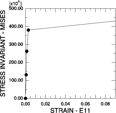
-
Click to close the dialog box.
-
It will also be helpful to display a symbol at each data point of the curve. Open the Curve Options dialog box.
-
From the Curves field, select the stress-strain curve (SVE11).
The SVE11 data object is highlighted.
-
Toggle on . Accept the defaults, and click at the bottom of the dialog box.
The stress-strain plot appears with a symbol at each data point of the curve.
You should now have a plot similar to the one shown in Figure 6. The stress-strain curve shows that the material behavior was linear elastic for this integration point during the first two increments of the simulation. In this plot it appears that the material remains linear during the third increment of the analysis; however, it does yield during this increment. This illusion is created by the extent of strain shown in the plot. If you limit the maximum strain displayed to 0.01 and set the minimum value to 0.0, the nonlinear material behavior in the third increment can be seen more clearly (see Figure 7).
Figure 7. Mises stress vs. direct strain (E11) along the lug in the corner element. Maximum strain 0.01.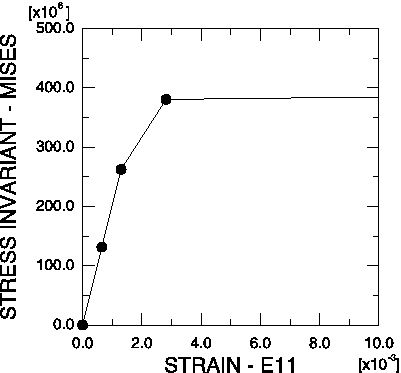
This stress-strain curve contains another apparent error. It appears that the material yields at 250 MPa, which is well below the initial yield stress. However, this error is caused by the fact that Abaqus/CAE connects the data points on the curve with straight lines. If you limit the increment size, the additional points on the graph will provide a better display of the material response and show yield occurring at exactly 380 MPa.
The results from this second simulation indicate that the lug will withstand this 60 kN load if the steel hardens after it yields. Taken together, the results of the two simulations demonstrate that it is very important to determine the actual post-yield hardening behavior of the steel. If the steel has very little hardening, the lug may collapse under the 60 kN load. Whereas if it has moderate hardening, the lug will probably withstand the load although there will be extensive plastic yielding in the lug (see Figure 3). However, even with plastic hardening, the factor of safety for this loading will probably be very small.
-