Contour integrals for a conical crack in a linear elastic infinite half space | ||
| ||
ProductsAbaqus/StandardAbaqus/CAE
Application description
This example examines the fracture behavior of a conical crack, which may result from a small hard object impacting a large brittle body. It shows how to evaluate the propensity of the crack to propagate under static loading but does not cover the event that formed the crack.
The J-integral is a widely applied fracture mechanics parameter that relates to energy release associated with crack growth and is a measure of the deformation intensity at a crack tip. In practice, the calculated J-integral can be compared with a critical value for the material under consideration to predict fracture. The T-stress represents stress parallel to the crack face. Together, the T-stress and the J-integral provide a two-parameter fracture model describing Mode I elastic-plastic crack-tip stresses and deformation in plane strain or three dimensions over a wide range of crack configurations and loadings. The stress intensity factors, , relate to the energy release rate and measure the propensity for crack propagation.
This example uses axisymmetric and three-dimensional models to demonstrate the Abaqus fracture mechanics capability, where the crack extension direction varies along a curved crack front. Submodeling and the use of infinite elements to simulate far-field boundaries are also demonstrated.
Geometry
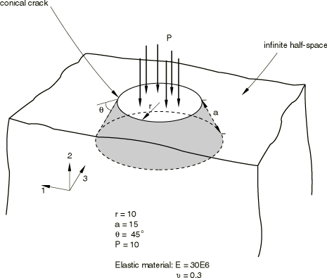
The problem domain contains a conical crack in an infinite solid half-space, as shown in Figure 1. The crack extension direction changes as the crack is swept around a circle. The units for this example are nonphysical; therefore, dimensions, loads, and material properties are described in terms of length and force units. The crack circumscribes a circle with a radius of 10 length units on the free surface. The crack intersects the free surface at 45° and extends 15 length units into the solid domain.
Materials
The material is a linear elastic solid.
Boundary conditions and loading
The semi-infinite domain is constrained from rigid body motion. The applied load is a static pressure with a magnitude of 10 force/length2 applied on the circular free surface of the block circumscribed by the crack. The loading is illustrated in Figure 1.
![]()
Abaqus modeling approaches and simulation techniques
This example includes six cases demonstrating different modeling approaches using Abaqus/Standard. The crack is modeled as a seam since the crack surfaces in the unloaded state lie next to one another with no gap.
The geometry is axisymmetric and can be modeled as such. However, the three-dimensional cases demonstrate the Abaqus fracture mechanics capability, where the crack extension direction varies along a curved crack front. The infinite half-space is treated using multiple techniques. In Case 1 through Case 4, the domain is extended well beyond the region of interest. Far-field boundary conditions applied a significant distance from the region of interest have negligible influence on the response near the crack. Cases 5 and Case 6 demonstrate the use of continuum infinite elements. Axisymmetric and three-dimensional cases are provided with and without submodeling. Fracture mechanics provides detailed information on fracture mechanics procedures.
Summary of analysis cases
| Case 1 | Full axisymmetric model using Abaqus/CAE. |
| Case 2 | Full three-dimensional model using Abaqus/CAE. |
| Case 3 | Axisymmetric approach with submodeling using Abaqus/CAE. |
| Case 4 | Three-dimensional approach with submodeling using Abaqus/CAE. |
| Case 5 | Axisymmetric approach with submodeling and infinite elements using input files. |
| Case 6 | Three-dimensional approach with submodeling and infinite elements using input files. |
The following sections discuss analysis considerations that are applicable to several or all the cases. More detailed descriptions are provided later including discussions of results and listings of files provided. The models for Case 1 through Case 4 were generated using Abaqus/CAE. In addition to the Python scripts that generate the model databases, Abaqus/Standard input files are also provided for those cases.
Mesh design
The mesh includes a seam along the crack with duplicate nodes, which allow the crack to open when loaded. The geometry is partitioned to map rings of elements around the crack tip for the contour integral calculations. The models use either quadrilateral or brick elements with a collapsed side to create triangular elements for two-dimensional cases or wedge-shaped elements for three-dimensional cases, which introduce a singularity at the crack tip. To be used for the evaluation of contour integrals, the mesh around the crack tip must be modeled as described in Using contour integrals to model fracture mechanics. In the axisymmetric cases a circular partition is created to mesh around the crack tip. In the three-dimensional cases the corresponding partition is a curved tubular volume enclosing the crack tip.
A refined mesh at the crack tip is required to obtain contour-independent results; i.e., there is no significant variation in the contour integral values calculated for successive rings of elements around the crack tip. In the circular partitioned region surrounding the crack tip where the contour integrals are calculated, the mesh should be biased moderately toward the crack tip. The accuracy of the contour integrals is not very sensitive to the biasing. Engineering judgment is required to establish adequate mesh refinement to produce contour-independent results while avoiding the possibility of creating elements at the crack tip that are so small in relation to other elements that they introduce numerical conditioning issues and associated round-off errors.
When the deformation and the material are linear as in this example, the diameter of the circular partition used to map the crack-tip mesh for contour integral calculations is not critical. (If the material is elastic-plastic, the size of the circular partition should generally contain the plastic zone and allow a number of the contours for the contour integrals to enclose the plastic zone while still remaining in the elastic region.) The remaining partitions are created so that the element shapes satisfy the element quality criteria in the regions away from the crack tip.
To understand the types of singularities created by collapsing the side of an element in two or three dimensions, see “Constructing a fracture mechanics mesh for small-strain analysis” in Contour integral evaluation. In this application we want to have a square root singularity in strain at the crack since the material is linear elastic and we will perform a small-strain analysis.
The stress intensity factors and the T-stresses are calculated using the interaction integral method, in which auxiliary plane strain crack-tip fields are employed. The crack front radius of curvature is significant for this problem. Therefore, to calculate the contour integrals accurately for the three-dimensional cases, a very refined mesh is used to approach the plane strain condition locally around the crack front. This refined mesh makes the contour integral domain sufficiently small to minimize the influence of curvature on the results.
Additional details of the meshing procedures for the axisymmetric and three-dimensional cases are discussed below within the descriptions of the individual cases.
Materials
The linear static structural analysis requires specification of Young’s modulus, which is 30,000,000 units of force/length2, and Poisson’s ratio, which is 0.3. One solid, homogenous section is used to assign material properties to the elements.
Loads
A uniform pressure load of 10 units of force/length2 is applied along the free top surface of the crack. In the axisymmetric models the load region, where the pressure is applied is represented by a line segment. For the three-dimensional cases the load region where the pressure is applied an area.
Analysis steps
Each analysis is performed using a single linear static step.
Output requests
Output requests are used to specify calculation of contour integrals, stress intensity factors, and T-stress. See Requesting contour integral output for more information regarding fracture mechanics output. The global models used in the submodeling cases include output requests necessary to write displacement and stress results to the output database (.odb) file; in the case where node-based submodeling is used, displacement results are used to establish boundary conditions on the corresponding submodels. In the case where surface-based submodeling is used, stress results are used to establish boundary tractions on the corresponding submodel.
Submodeling
Realistic fracture analyses tend to require significant computer resources. To obtain accurate results when analyzing the stress field around a crack tip, a refined mesh must be used to capture the strong gradients near the tip. The required mesh refinement can make fracture mechanics models large since a crack is normally a very small feature compared with the model dimensions. An alternative technique that reduces computational resources is to use submodeling to obtain accurate results by running two smaller models sequentially instead of performing a single global analysis with a refined mesh around the crack. The first step is to solve a less refined global model to obtain a solution that is accurate away from the crack tip but is not sufficiently refined to capture strong gradients near the region of interest. A refined submodel of the crack-tip region is then used to obtain a more accurate solution and, hence, more accurate contour integrals. The boundaries of the submodel must be far enough from the region of interest that the less refined global model is able to provide accurate results at the submodel boundaries, particularly important when surface-based submodeling is used. This condition is verified during postprocessing by confirming that the stress contours at the boundaries of the submodel are similar to the stress contours at the same location in the global model.
Although the submodeling approach is not required for this example because the refined models for the entire domain analyzed in Case 1 and Case 2 are small enough to run on commonly available computing platforms, this application provides an opportunity to demonstrate submodeling techniques for both axisymmetric and three-dimensional fracture mechanics cases, as well as showing the differences between node-based submodeling based on displacements and surface-based submodeling based on stresses. Submodeling procedures are described in detail in Node-based submodeling, Surface-based submodeling, and Submodeling.
Modeling an infinite domain
Case 1 through Case 4 simulate the infinite extent of the domain with a continuum mesh that is large compared to the crack dimensions with appropriate far-field boundary conditions. In those cases the domain extends 20 times the crack length. Case 5 and Case 6 demonstrate the use of continuum infinite elements and represent the region of interest with reduced-integration continuum elements to a distance approximately 10 times the crack dimensions surrounded by a layer of continuum infinite elements. Far-field boundary conditions are not required in these cases.
![]()
Case 1 Full axisymmetric model with Abaqus/CAE
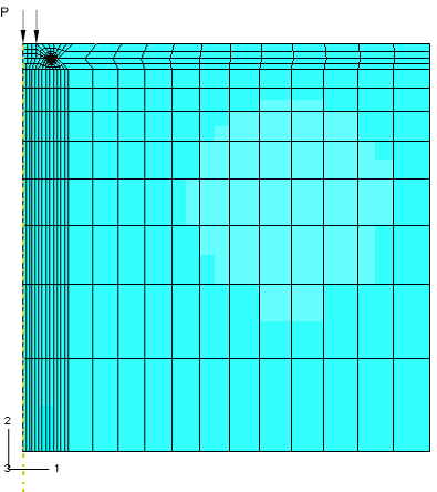
The axisymmetric domain is a solid with a radius equal to the height of 300 length units (see Figure 2). The top edge of the model represents the free surface containing the crack. The semi-infinite domain is simulated by extending the continuum model to a distance 20 times the length of the crack and applying appropriate far-field boundary conditions. This model uses continuum axisymmetric quadratic reduced-integration (CAX8R) elements.
Mesh design
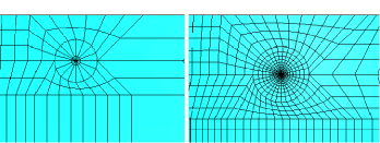
When calculating contour integrals in two-dimensional problems, quadrilateral elements must be used around the crack tip where the contour integral calculations will be performed with triangular elements adjacent to the crack tip. These triangular elements are actually collapsed quadrilaterals, which introduce a singularity. The axisymmetric model must be partitioned as shown in Figure 2 to define the crack, introduce a singularity by collapsing elements at the crack tip, and create rings of quadrilateral elements for contour integral calculations. A straight line partition is created where the seam crack is defined along with a circular partition, which enables mapping rings of elements around the crack tip. When structured meshing is used for this partition, triangular elements are created adjacent to the crack tip with quadrilaterals surrounding them (see Using contour integrals to model fracture mechanics). Abaqus/CAE automatically converts triangular elements at the crack tip to quadrilaterals with one side collapsed to introduce a singularity.
Creating a seam describes how to pick partition segments to define the seam (crack). Procedures to create a square root singularity in strain at the crack tip are described in Controlling the singularity at the crack tip. After defining the seam, pick the crack tip to specify the region defining the first contour integral and define the q vector to specify the crack extension direction as described in Creating a contour integral crack.
Boundary conditions
The right edge of the model shown in Figure 3 is unconstrained to represent the far-field boundary. The bottom edge of the model is constrained to zero displacement (U2) to eliminate rigid body motion while simulating the far-field boundary. These edges are far enough away from the area of interest around the crack to represent an infinite domain with negligible influence on the area of interest.
Run procedure
The Case 1 model is generated using Abaqus/CAE to create and to mesh native geometry. Python scripts are provided to automate building the model and running the solution. The scripts can be run interactively or from the command line.
To create the model interactively, start Abaqus/CAE and select from the Start Session dialog box that appears. Select the first file for the case, AxisymmConeCrack_model.py. When the script completes, you can use Abaqus/CAE commands to display and to query the model. When you are ready to analyze the model, select from the menu and choose the next script, AxisymmConeCrack_job.py. The Python scripts provided allow you to modify the model interactively with Abaqus/CAE to explore additional variations on the cases provided here.
Alternatively, the Python scripts can be run from the command line with the Abaqus/CAEnoGUI option in the order listed:
abaqus cae noGUI=filename.py where abaqus is the system command to run the program and filename is the name of the script to be run.
As an alternative to the Python scripts, an Abaqus/Standard input file AxisymmConeCrack.inp is also provided to run this case. You can submit the analysis using the input file with the following command:
abaqus input=AxisymmConeCrack.inp
![]()
Case 2 Full three-dimensional model with Abaqus/CAE
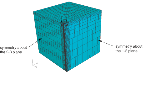
The three-dimensional domain is a cube with an edge length of 300 units, as shown in Figure 4. The mesh represents a quarter-symmetric segment of the problem domain. The top of the model represents the free surface containing the crack. The semi-infinite domain is represented by extending the continuum mesh to a distance 20 times the length of the crack with appropriate symmetry and far-field boundary conditions.
Mesh design
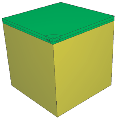
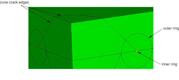
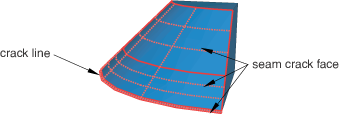
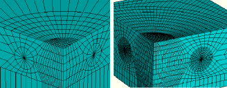
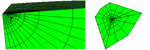
When calculating three-dimensional contour integrals, rings of brick elements must be used around the crack tip where the contour integral calculations will be performed with wedge elements adjacent to the crack tip (these wedges are actually collapsed bricks). Concentric tubular partitions are created to map the mesh around the crack tip. The three-dimensional domain and partitioning of the geometry are illustrated in Figure 5 and Figure 6. The seam crack is shown in Figure 7. When structured meshing is used for the inner tubular partition, wedge elements are created adjacent to the crack tip with rings of bricks surrounding them (see Using contour integrals to model fracture mechanics for details). A swept mesh used in the inner ring creates wedge elements at the crack tip. The outer ring is meshed with hexahedral elements using the structured meshing technique.
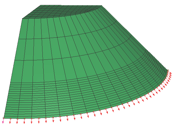
For details on how to define the crack propagation direction where the direction of the vectors varies along the crack front (referred to as the q vector), see Defining the crack extension direction. Figure 8 illustrates the q vectors.
Boundary conditions
Symmetric displacement boundary conditions are applied normal to the symmetry planes. The far-field faces on the sides of the model, which are not symmetry planes, are unconstrained. The bottom face of the model is constrained from displacement in the direction of the pressure load (U2=0) to prevent rigid body motion while simulating a far-field boundary condition.
Run procedure
The Python scripts provided to generate the Abaqus/CAE model and to analyze the model are run following the same procedures as those described for Case 1.
As an alternative to the Python scripts, an Abaqus/Standard input file SymmConeCrackOrphan.inp is also provided to run this case. You can submit the analysis using the input file with the following command:
abaqus input= SymmConeCrackOrphan.inp
The files defining nodes and elements for this case, SymmConeCrackOrphan_node.inp and SymmConeCrackOrphan_elem.inp, must be available when the input file is submitted.
Figure 9 shows a deformed shape plot for the three-dimensional model of the crack from the full three-dimensional analysis of Case 2. The displacement is exaggerated using a scaling factor to visualize the crack opening.
![]()
Case 3 Axisymmetric approach with submodeling using Abaqus/CAE
Case 3 uses the submodeling approach and, hence, requires two sequential analyses, which are referred to as the global model and the submodel. First, a less refined global model is solved to obtain the displacement solution with sufficient accuracy away from the crack tip. A refined submodel of the area of interest driven by the displacement solution from the global model is then used to obtain an accurate solution in the crack-tip region. Each of these models is much smaller than the fully refined axisymmetric global model used in Case 1.
Mesh design
The axisymmetric global model has a relatively less refined mesh in the crack region. The global model used for Case 3 has two rings of elements where the mesh focuses on the crack tip, compared to 13 rings of elements around the crack tip in the full model used in Case 1.
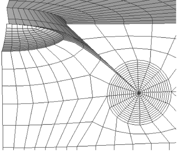
The axisymmetric global model and the submodel meshes for Case 3 are shown in Figure 10. The axisymmetric submodel has a refined mesh around the crack tip with 12 rings of elements surrounding the crack tip. It is assumed that the global model’s coarse mesh is sufficiently accurate to drive the submodel: the submodel can obtain accurate contour integral results if the global model's displacement field is accurate at the boundaries of the submodel, which lie far from the crack tip. You can verify this at the postprocessing stage by comparing stress contours at the boundaries of the submodel to the corresponding contours of the global model.
Boundary conditions
The boundary conditions applied to the axisymmetric global model are the same as those used in Case 1. The displacement solution from the global model is applied to the submodel boundaries when the submodeling technique is used.
Run procedure
The models used for Case 3 are generated using Abaqus/CAE to create and to mesh native geometry. The same procedures used to run the Python scripts for Cases 1 and 2 are used to create and to analyze the global model. The script that builds the submodel refers to the global model output database (.odb) file, which must be available when the submodel is analyzed. After analyzing the global model, run the scripts to build and to analyze the submodel using the same procedure used for the global model.
Abaqus/Standard input files are also provided to run this case. First, run the job to create and to analyze the global model; then run the submodel job. The results from the global model must be available to run the submodel. A typical execution procedure is as follows:
abaqus job=globalModelJobName  input=globalModelInputfile.inp
abaqus job=submodelJobname, input=subModelInputfile.inp,
globalmodel=globalModelJobNameOutputDatabase
![]()
Case 4 Three-dimensional approach with submodeling using Abaqus/CAE
Case 4 uses a three-dimensional submodeling approach and requires two sequential analyses, a global model and a submodel. First, a global model is solved with sufficient refinement to provide an accurate displacement and stress solution away from the crack tip.
Two versions of refined submodels of the area of interest are then used to obtain an accurate solution in the crack-tip region. In one submodel analysis the area of interest is driven by the displacement solution from the global model. In the other submodel analysis the area of interest is driven by the stress solution from the global model.
Each of the models used in this case is much smaller than the fully refined three-dimensional global model used in Case 2.
Mesh design
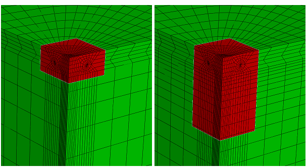
The three-dimensional global model, with a less refined mesh in the crack region, is first analyzed and then used to drive the submodel. For the three-dimensional global model only 18 elements are used along the crack line, whereas 38 elements are used along the crack line in the submodel. Figure 11 shows the meshes for the three-dimensional global model and the submodel.
Boundary conditions
The boundary conditions applied to the global model in Case 4 are the same as those used in the full three-dimensional Case 2. The submodeling approach uses either the displacement or stress solution from the global model to drive the submodel boundaries.
Run procedure
The models used for Case 4 are generated using Abaqus/CAE to create and to mesh native geometry. The same procedures used to run Case 3 can be used with Case 4. The script that builds the submodel refers to the global model output database (.odb) file, which must be available when the submodel is analyzed.
As an alternative to the Python scripts, Abaqus/Standard input files are also provided to run this case. These are submitted using the same procedure described for the input files under Case 3.
![]()
Case 5 Axisymmetric submodeling approach with infinite elements using Abaqus/Standard input files
Case 5 uses the submodeling approach with an axisymmetric mesh utilizing continuum infinite elements to simulate the far-field boundary condition. The submodeling technique requires two sequential analyses, a less refined global model and a refined submodel at the crack tip.
The global model in Case 5 comprises an axisymmetric representation of the hemispherical domain with continuum elements to a radius of 170 length units. Eight-node biquadratic axisymmetric quadrilateral, reduced-integration elements (CAX8R) are used to model the solid domain in the region adjacent to the crack. The domain is further extended using a layer of continuum infinite elements to a radius of 340 length units. Five-node quadratic axisymmetric one-way infinite elements (CINAX5R) are used to simulate the far-field region of the solid. The submodel used in Case 5 does not encompass the complete crack face but extends to a distance far enough from the crack tip that strong variations in the stress field are captured within the submodel. This result can be verified by comparing stress contours of the submodel with the corresponding stress contours in the global model.
Mesh design
The axisymmetric global model, with a relatively less refined mesh in the crack region, is first analyzed and then used to drive the submodel. The axisymmetric global model and the submodel meshes for Case 5 are shown in Figure 12.
Boundary conditions
The continuum infinite elements eliminate the need for far-field constraints, which were required in Case 1 through Case 4.
Run procedure
The models used for Case 5 are generated using Abaqus/Standard input files. First, run the job to create and to analyze the global model; then run the submodel job. The results from the global model must be available to run the submodel. A typical execution procedure is as follows:
abaqus job=globalModelJobName  input=globalModelInputfile.inp
abaqus job=submodelJobname, input=subModelInputfile.inp,
globalmodel=globalModalJobNameOutputDatabase
![]()
Case 6 Three-dimensional approach with infinite elements using submodeling with Abaqus/Standard input files
Case 6 uses the submodeling approach with a three-dimensional mesh utilizing continuum infinite elements to simulate the far-field boundary condition. The domain modeled for Case 6 encompasses an eighth of a sphere, representing one-quarter of the semi-infinite problem domain. Continuum elements are used to a radius of 170 length units. The domain is extended using a layer of infinite continuum elements to a radius of 340 length units.
The submodeling technique requires two separate analyses, a less refined global model and a refined submodel at the crack tip. Case 6 uses Abaqus/Standard input files to generate the models rather than Abaqus/CAE Python scripts. Twenty-node quadratic, reduced-integration solid elements (C3D20R) are used to model the solid domain in the region adjacent to the crack. The domain is further extended using a layer of 12-node quadratic one-way infinite brick elements (CIN3D12R) to a radius of 340 length units.
The submodel used in Case 6 does not encompass the complete crack face but extends to a distance far enough from the crack tip that strong variations in the stress field are captured within the submodel.
Mesh design
The three-dimensional global model, with a relatively less refined mesh in the crack region, is first analyzed and then used to drive the submodel. The three-dimensional global model and the submodel meshes for Case 6 are shown in Figure 13.
Boundary conditions
The continuum infinite elements eliminate the need for far-field constraints, which were required in Case 1 through Case 4.
Run procedure
The models of Case 6 are generated using Abaqus/Standard input files. The same procedure used in Case 5 is also used in Case 6. The files containing the node and element definitions for the three-dimensional global model must be available when the input file is run to create the global model . The output database (.odb) file from the global model must be available to run the submodel.
![]()
Discussion of results and comparison of cases
Contour integral results obtained from the data (.dat) file for each case are summarized in Table 1 through Table 4. These results are also available from the output database (.odb) file by displaying history output in the Visualization module of Abaqus/CAE. While there is no analytical solution available for comparison, an additional axisymmetric analysis with extreme mesh refinement is used as the basis for a reference solution. Each table includes the reference solution value in the table title.
Abaqus calculates the J-integral using two methods. Values of the J-integral are based on the stress intensity factors, JK, and by evaluating the contour integral directly, JA. The stress intensity factors and , and the T-stresses are given in Table 2, Table 3, and Table 4, respectively. When the stress intensity factors are requested, Abaqus automatically outputs the J-integrals based on the stress intensity factors, JK. Values of are not tabulated because these values should equal zero based on the loading and are negligibly small relative to and .
The tables list values for contour 1 through contour 5. Each contour corresponds to a successive ring of elements progressing outward radially from the crack tip. For the axisymmetric cases one set of results is available for each contour. For the three-dimensional cases Abaqus/Standard provides contour integral values at each crack-tip node. The values listed in Table 1 through Table 4 for the three-dimensional cases correspond to the location halfway along the circumference of the crack, which lies midway between the symmetry faces of the three-dimensional models. A detailed examination of the results for the three-dimensional cases confirms that the contour integral values are essentially constant at each node along the circumference of the crack tip. The exception is the value calculated for ; which fluctuates but remains small relative to and over almost the full length of the crack; however increases at the open end faces of the crack corresponding to the symmetry planes. A loss of accuracy occurring at the node corresponding to the open end of a three-dimensional crack is a known limitation that can be expected when applying this method.
Results from the first contour are generally not used when evaluating fracture problems because the first contour is influenced by the singularity associated with the crack tip. The average quantities reported in the tabular results exclude the first contour. Comparisons refer only to contour 2 through contour 5. The axisymmetric and the three-dimensional modeling approaches are in close agreement, with and without submodeling. For each case, values of the tabulated quantities for J calculated by evaluating the contour integrals directly, (JA), , , and T-stresses deviate by less than 2% of the average of the corresponding values for contour 2 through contour 5. The J-integral for each case, calculated from the stress intensity factors (JK) deviate by less than 3.5% of the average of corresponding values. The larger deviation for JK versus JA is expected because the method of calculating contour integrals from the stress intensity factors (JK) is more sensitive to numerical precision than calculating the contour integrals directly (JA). is analytically equal to zero due to the geometry and loading symmetry in this example; the numerical results for are negligibly small relative to and .
Submodeling results
The global models used to calculate the deformation and stress fields that drive the submodels use crack-tip meshes that are too coarse to give accurate results for the contour integrals; therefore, the results for the global models are not tabulated. Results are tabulated for the submodels that refer to this global analysis. Generally these results verify that the submodeling approach provides adequate accuracy in fracture problems where it may not be practical to use a sufficiently refined mesh in the crack-tip region of a global model. The node-based submodeling approach provides greater accuracy than the surface-based approach.
Node-based submodeling results
The J-integral values for the node-based submodel analyses match those for the full model analyses (analyses with adequate mesh refinement around the crack tip) to within less than 1%.
Surface-based submodeling results
The three-dimensional submodeling case also considers surface-based submodeling, where the submodel is driven by the global model stress field. Two different pairs of global models and surface-based submodels are considered: one that matches the mesh design used in the node-based analysis, and one where adjustments are made to improve accuracy. The J-integral values for the first analysis pair, with the same meshes as in node-based submodeling, match those for the full model only to within 6%. These inaccurate results arise from a modeling arrangement that violates guidelines established in Surface-based submodeling, namely that
the submodel surface should intersect the global model in regions of relatively low stress gradients, and
the submodel surface should intersect the global model in regions of uniform element size.
Adjusted global and submodel analyses that adhere to these guidelines are run. In this case the submodel driven surface is farther from the crack region and the high stress gradient, and the global model mesh is refined so that elements are more uniform in the region of the submodel surface. Figure 14 shows a comparison of the submodel/global model pairs. The modeling arrangement on the left places the lower submodel boundary too near to the crack and high stress gradients and cuts through high aspect ratio elements. The arrangement on the right provides lower aspect ratio elements in the global model and positions the lower submodel boundary further from the crack. The adjusted analysis with the further boundary now matches the J-integral values for the full model to within 2%. This accuracy difference illustrates the importance of adhering to the guidelines for surface-based submodel design. In practice, in the absence of a reference global solution, you should use the following guidelines to ensure your surface-based solution is adequate:
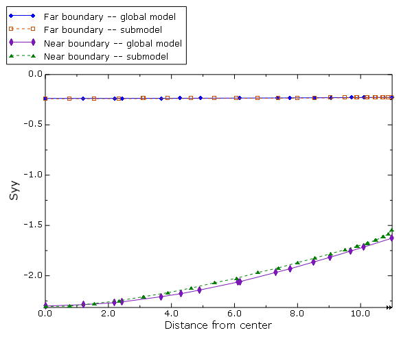
As with any submodel analysis, compare solution results between the global model and submodel on the submodel boundary. In this case a stress comparison is appropriate. Figure 15 compares the 2-component of stress for the two surface-based submodel analyses and their corresponding global model. Results are plotted on a path lying in the lower submodel boundary and extending from the center radially outward. The near-boundary submodel has a significantly greater stress discrepancy with the global model.
In cases where inertia relief is employed to address rigid body modes in surface-based submodeling, if the inertia relief force output variable (IRF) is small compared to the prevailing force level in the model, the surface-based stress distribution is equilibrated. In this model the prevailing force is the 10 units of pressure acting on the surface circumscribed on the crack (a radius of 6), or 786 units of force for the three-dimensional quarter symmetry model.
In this analysis the inertia relief force in the 2-direction is similar in both cases (33 for the near-boundary model and 32 for the far-boundary model) and relatively small; hence, in this case, the inertia relief force would not suggest poorer results with the near-boundary submodel, and its small value is not a sufficient measure of the adequacy of the submodel design.
![]()
Files
You can use the Python scripts for Abaqus/CAE and input files for Abaqus/Standard to create and to run the cases.
Case 1 Full axisymmetric analysis
- AxisymmConeCrack_model.py
Script to create the model, including instructions for creating the mesh used for the reference solution.
- AxisymmConeCrack_job.py
Script to analyze the model.
- AxisymmConeCrack.inp
Input file to create and to analyze the model.
Case 2 Full three-dimensional model
- SymmConeCrack_model.py
Script to create the model.
- SymmConeCrack_job.py
Script to analyze the model.
- SymmConeCrackOrphan.inp
Input file to create and to analyze the model.
- SymmConeCrackOrphan_node.inp
Nodes for SymmConeCrackOrphan.inp.
- SymmConeCrackOrphan_elem.inp
Elements for SymmConeCrackOrphan.inp.
Case 3 Axisymmetric submodel analysis
- AxisymmConeCrackGl_model.py
Script to create the model.
- AxisymmConeCrackGl_job.py
Script to analyze the model and to create the output database file that drives the submodel.
- AxisymmConeCrackSub_model.py
Script to create the submodel.
- AxisymmConeCrackSub_job.py
Script to analyze the submodel using the results from the global model output database file to drive it.
- AxisymmConeCrackGl.inp
Input file to create and to analyze the global model.
- AxisymmConeCrackSub.inp
Input file to create and to analyze the submodel.
Case 4 Three-dimensional submodel analysis
- SymmConeCrackGl_model.py
Script to create the global model.
- SymmConeCrackGl_job.py
Script to analyze the global model and to create the output database file that drives the submodel. Refer to parameter definitions in the script to create the adjusted global model referred to in Submodeling results.
- SymmConeCrackSub_model.py
Script to create the node-based submodel.
- SymmConeCrackSub_job.py
Script to analyze the node-based submodel using the results from the global model output database file to drive it.
- SymmConeCrackSubSb_near_model.py
Script to create the surface-based submodel.
- SymmConeCrackSubSb_near_job.py
Script to analyze the surface-based submodel using the stress results from the global model output database file to drive it.
- SymmConeCrackSubSb_far_model.py
Script to create the surface-based submodel with a far-boundary submodel.
- SymmConeCrackSubSb_far_job.py
Script to analyze the surface-based submodel with the far-boundary submodel using the stress results from the global model output database file to drive it.
- SymmConeCrackGlOrphan.inp
Input file to create and to analyze the global model.
- SymmConeCrackGlOrphan_node.inp
Nodes for SymmConeCrackGlOrphan.inp.
- SymmConeCrackGlOrphan_elem.inp
Elements for SymmConeCrackGlOrphan.inp.
- SymmConeCrackGlOrphanAdj.inp
Input file to create and to analyze the global model that is adjusted for improved surface-based submodel accuracy.
- SymmConeCrackGlOrphanAdj_node.inp
Nodes for SymmConeCrackGlOrphanAdj.inp.
- SymmConeCrackGlOrphanAdj_elem.inp
Elements for SymmConeCrackGlOrphanAdj.inp.
- SymmConeCrackSubOr.inp
Input file to create and to analyze the node-based submodel.
- SymmConeCrackSubOr_node.inp
Nodes for SymmConeCrackSubOr.inp.
- SymmConeCrackSubOr_elem.inp
Elements for SymmConeCrackSubOr.inp.
- SymmConeCrackSubOrSb_near.inp
Input file to create and to analyze the submodel using the surface-based submodel technique to drive the submodel stresses.
- SymmConeCrackSubOrSb_near_node.inp
Nodes for SymmConeCrackSubOrSb_near.inp.
- SymmConeCrackSubOrSb_near_elem.inp
Elements for SymmConeCrackSubOrSb_near.inp.
- SymmConeCrackSubOrSb_far.inp
Input file to create and to analyze the submodel with the far-boundary submodel using the surface-based submodel technique to drive the submodel stresses.
- SymmConeCrackSubOrSb_far_node.inp
Nodes for SymmConeCrackSubOrSb_far.inp.
- SymmConeCrackSubOrSb_far_elem.inp
Elements for SymmConeCrackSubOrSb_far.inp.
Case 5 Axisymmetric submodel analysis using infinite continuum elements
- conicalcrack_axiglobal.inp
Input file to analyze the axisymmetric global model and to create the output database file that drives the submodel.
- conicalcrack_axisubmodel_rms.inp
Input file to analyze the axisymmetric submodel using the results from the global model output database file to drive it.
Case 6 Three-dimensional submodeling analysis using infinite continuum elements
- conicalcrack_3dglobal.inp
Input file to analyze the three-dimensional global model and to create the output database file that drives the submodel.
- conicalcrack_3dsubmodel_rms.inp
Input file to analyze the three-dimensional submodel using the results from the global model output database file to drive it.
![]()
References
, , and , “Energy Release Rate Along a Three-Dimensional Crack Front in a Thermally Stressed Body,” International Journal of Fracture, vol. 30, pp.79–102, 1986.
![]()
Tables
| Solution | Contour | Average Value, Contours 2–5 | |||||
|---|---|---|---|---|---|---|---|
| Jestimate method | 1 | 2 | 3 | 4 | 5 | ||
| Case 1: Full axisymmetric | JK | 1.326 | 1.308 | 1.288 | 1.262 | 1.228 | 1.272 |
| JA | 1.334 | 1.333 | 1.334 | 1.334 | 1.334 | 1.334 | |
| Case 2: Full three-dimensional | JK | 1.303 | 1.325 | 1.312 | 1.295 | 1.274 | 1.302 |
| JA | 1.308 | 1.334 | 1.336 | 1.337 | 1.337 | 1.336 | |
| Case 3: Submodel axisymmetric | JK | 1.327 | 1.319 | 1.311 | 1.300 | 1.287 | 1.304 |
| JA | 1.330 | 1.329 | 1.330 | 1.330 | 1.330 | 1.330 | |
| Case 4: Node-based submodel three-dimensional | JK | 1.314 | 1.316 | 1.303 | 1.285 | 1.264 | 1.292 |
| JA | 1.318 | 1.326 | 1.328 | 1.328 | 1.328 | 1.328 | |
| Case 4: Surface-based submodel three-dimensional | JK | 1.396 | 1.398 | 1.385 | 1.367 | 1.345 | 1.374 |
| JA | 1.400 | 1.408 | 1.409 | 1.408 | 1.407 | 1.408 | |
| Case 4: Surface-based submodel with far boundary, three-dimensional | JK | 1.345 | 1.347 | 1.335 | 1.317 | 1.296 | 1.324 |
| JA | 1.349 | 1.357 | 1.359 | 1.358 | 1.358 | 1.358 | |
| Case 5: Submodel axisymmetric with infinite elements | JK | 1.413 | 1.359 | 1.363 | 1.363 | 1.361 | 1.362 |
| JA | 1.407 | 1.360 | 1.365 | 1.365 | 1.365 | 1.364 | |
| Case 6: Submodel three-dimensional with infinite elements | JK | 1.329 | 1.363 | 1.367 | 1.368 | 1.368 | 1.367 |
| JA | 1.336 | 1.361 | 1.366 | 1.366 | 1.366 | 1.365 | |
| Solution | Contour | Average Value, Contours 2–5 | ||||
|---|---|---|---|---|---|---|
| 1 | 2 | 3 | 4 | 5 | ||
| Case 1: Full axisymmetric | 0.495 | 0.497 | 0.499 | 0.500 | 0.499 | 0.499 |
| Case 2: Full three-dimensional | 0.492 | 0.501 | 0.503 | 0.502 | 0.500 | 0.502 |
| Case 3: Submodel axisymmetric | 0.491 | 0.493 | 0.494 | 0.495 | 0.496 | 0.494 |
| Case 4: Node-based submodel three-dimensional | 0.491 | 0.496 | 0.498 | 0.497 | 0.494 | 0.497 |
| Case 4: Surface-based submodel three-dimensional | 0.426 | 0.431 | 0.433 | 0.431 | 0.427 | 0.430 |
| Case 4: Surface-based submodel with far boundary, three-dimensional | 0.436 | 0.441 | 0.443 | 0.442 | 0.439 | 0.441 |
| Case 5: Submodel axisymmetric with infinite elements | 0.537 | 0.527 | 0.528 | 0.528 | 0.529 | 0.528 |
| Case 6: Submodel three dimensional with infinite elements | 0.522 | 0.528 | 0.529 | 0.530 | 0.530 | 0.528 |
| Solution | Contour | Average Value, Contours 2–5 | ||||
|---|---|---|---|---|---|---|
| 1 | 2 | 3 | 4 | 5 | ||
| Case 1: Full axisymmetric | –2.032 | –2.016 | –2.000 | –1.978 | –1.949 | –1.986 |
| Case 2: Full three-dimensional | –2.013 | –2.029 | –2.018 | –2.004 | –1.987 | –2.010 |
| Case 3: Submodel axisymmetric | –2.033 | –2.026 | –2.019 | –2.010 | –1.999 | –2.014 |
| Case 4: Node-based submodel three-dimensional | –2.023 | –2.023 | –2.012 | –1.997 | –1.980 | –2.003 |
| Case 4: Surface-based submodel three-dimensional | –2.102 | –2.103 | –2.092 | –2.078 | –2.061 | –2.084 |
| Case 4: Surface-based submodel with far boundary, three-dimensional | –2.060 | –2.060 | –2.050 | –2.036 | –2.019 | –2.041 |
| Case 5: Submodel axisymmetric with infinite elements | –2.090 | –2.050 | –2.053 | –2.052 | –2.051 | –2.051 |
| Case 6: Submodel three dimensional with infinite elements | 2.027 | 2.053 | 2.057 | 2.057 | 2.057 | 2.056 |
| Solution | Contour | Average Value, Contours 2–5 | ||||
|---|---|---|---|---|---|---|
| 1 | 2 | 3 | 4 | 5 | ||
| Case 1:Full axisymmetric | –0.982 | –0.979 | –0.976 | –0.972 | –0.967 | –0.973 |
| Case 2: Full three-dimensional | –0.942 | –0.972 | –0.966 | –0.960 | –0.954 | –0.963 |
| Case 3:Submodel Axisymmetric | –0.980 | –0.978 | –0.977 | –0.975 | –0.973 | –0.976 |
| Case 4: Node-based submodel three-dimensional | –0.947 | –0.966 | –0.959 | –0.953 | –0.947 | –0.956 |
| Case 4: Surface-based submodel three-dimensional | –0.981 | –0.996 | –0.989 | –0.983 | –0.976 | –0.986 |
| Case 4: Surface-based submodel with far boundary, three-dimensional | –0.958 | –0.973 | –0.966 | –0.960 | –0.954 | –0.963 |
| Case 5: Submodel axisymmetric with infinite elements | –1.182 | –0.983 | –0.985 | –0.984 | –0.984 | –0.984 |
| Case 6: Submodel three-dimensional with infinite elements | –0.599 | –0.982 | –0.984 | –0.983 | –0.982 | –0.982 |
![]()
Figures
