Using the adaptivity plotter plug-in | ||
| ||
Select the desired adaptivity process from the model database.
Toggle on the remeshing rules that you want to plot. Where applicable, you can choose the following:
The error indicators generated by the remeshing rule.
The global norms of these error indicators.
Toggle on Plot in separate viewport to create a new viewport for the X–Y plot. If you leave this option toggled off, the plug-in will create the X–Y plot in the current viewport.
Toggle on Show element count to plot the element count, totaled over all the active remeshing rules.
Toggle on Show remeshing rule targets to plot the target error indicator norm for each rule.
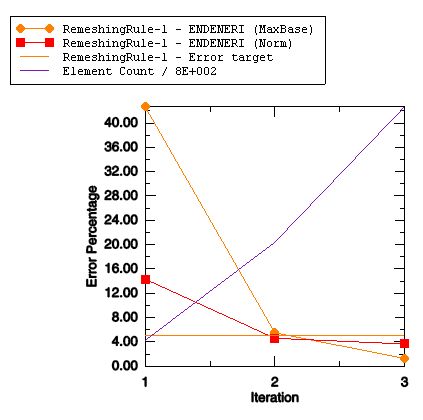
Click to create the X–Y plot, or click to create a table of the error indicator norms in HTML format. An example of an X–Y plot created by the plug-in is shown in Figure 1.
Figure 1. An X–Y plot created by the Adaptivity Plotter plug-in.
The following four values are plotted in Figure 1:
The MaxBase norm for the error indicator ENDENERI for RemeshingRule-1. This norm represents the error indicator value at the location of maximum energy density, normalized by that density.
The global Norm for the error indicator ENDENERI for RemeshingRule-1. This norm represents a normalized average of the error indicator over the entire remeshing rule domain.
The error target, which is the target set when you create the remeshing rule. In this example the target is fixed at 5%.
The element count, representing the sum of elements in each of the active remeshing rule regions. The Y-axis scale is percent, which is used by the plots of error indicator and error target. To determine the error count, you must multiply the scaling factor indicated in the legend, 800 in this example, by the percent value on the Y-axis. For example, the element count at iteration 2 is approximately 20 × 800, or 16000 elements.