Uniformly loaded, elastic-plastic plate

This example verifies the application of a standard rate-independent plasticity theory for metals and assesses the accuracy of the integration of the plasticity equations, especially in the case of nonproportional stressing.

Integration of elastic-plastic material models is a potential source of error in numerical structural analysis. See, for example, the discussions by Krieg and Krieg (1977) and Schreyer et al. (1979). Usually the error is most severe when kinematic hardening is used in plane stress with nonproportional stressing (perhaps because of the complexity of the motion of the stress point and yield surface in stress space in this theory). This example contains two such problems for which the exact solutions are available (Foster Wheeler report, 1972). Experience with a number of other computer programs has suggested that the second example, in particular, is a severe test of the numerical implementation of the plasticity theory. Both problems involve states of uniform plane stress and, hence, are done here by using a single plane stress element.

The following topics are discussed:

Problem description
Model and loading
Results and discussion
Input files
References
Tables
Figures

ProductsAbaqus/Standard

Problem description

The material models for the unixially and biaxially loaded cases are described below.

Case 1—Uniaxial loading

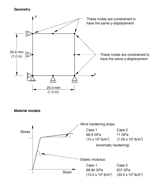
Figure 1 shows the material model for this case. The elastic modulus is 68.94 GPa (10.0 × 10⁶ lb/in²), the yield stress is 68.9 MPa (10.0 × 10³ lb/in²), and the work hardening slope is 68.9 GPa (10.0 × 10⁶ lb/in²). This is specified by giving a yield stress of 34.57 GPa (5.01 × 10⁶ lb/in²) at a plastic strain of 0.5. The total force and the total moment on the loaded face of the model are output to the results file.

Case 2—Biaxial loading

Figure 1 shows the material model for this case. The elastic modulus is 207 GPa (30.0 × 10⁶ lb/in²), the yield stress is 207 MPa (30.0 × 10³ lb/in²), and the work hardening slope is 11 GPa (1.59 × 10⁶ lb/in²). This is specified by giving a yield stress of 10.62 GPa (1.53 × 10⁶ lb/in²) at a plastic strain of 0.95.

Model and loading

The geometries and loading distributions for the unixial and biaxial cases are described below.

Case 1—Uniaxial loading

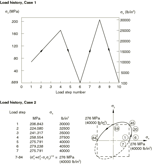
Figure 1 shows the geometry for this case. Two types of meshes are provided: a single-element mesh using higher-order plane stress and shell elements (CPS8R, S8R5, S9R5, and STRI65) and a mesh using linear shell and continuum shell elements (S4R and SC8R). Two edges have simple support. The load history is shown in Figure 2 and is prescribed with an amplitude curve (Amplitude Curves). The load distribution is a uniform, direct stress on the element edge. Since the strain should be uniform, the edge nodes are constrained using an equation constraint (Linear constraint equations) to move together in the direction normal to the edge. Then the total load on the edge is simply given on one of the edge nodes.

Case 2—Biaxial loading

The case is set up with the same geometric model (Figure 1). However, the loading is more complex (see Figure 2).

First, the plate is loaded into the plastic range in uniaxial tension in the x-direction, unloaded slightly, and reloaded. Biaxial loading then follows, with $σ_{x}$ and $σ_{y}$ prescribed, as shown in Figure 2, so that the quantity $\sqrt{σ_{x}^{2} + σ_{y}^{2} - σ_{x} σ_{y}}$ remains constant at 276 MPa (40000 lb/in²). This loading is defined by an amplitude curve by reading in a file of values previously calculated in the small program AMP (see elasticplasticplate_amplitude.f).

Results and discussion

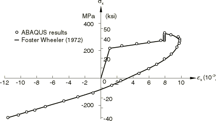
Exact solutions for these two problems have been developed by Chern in a Foster Wheeler report (1972), where they are documented as Problems 8 and 9. These solutions provide a basis for the comparison of the Abaqus results.

Case 1—Uniaxial loading

The plastic strains are the basic solution in these cases (since stress is prescribed). The results for this case are summarized in Table 1. The Abaqus results agree with the exact solution. Table 1 also records the number of iterations required to achieve equilibrium.

Case 2—Biaxial loading

The results in this case are best represented by the $σ_{x}$ versus $ε_{x}$ plot shown in Figure 3. The agreement with the exact solution is again very close.

Input files

elasticplasticplate_cps8r_uni.inp: Uniaxial loading case using the CPS8R element.
elasticplasticplate_cps8r_bi.inp: Biaxial loading case using the CPS8R element.
elasticplasticplate_amplitude.f: Program used to generate the amplitude data records.
elasticplasticplate_s8r5_uni.inp: Uniaxial loading case using the S8R5 element.
elasticplasticplate_s8r5_bi.inp: Biaxial loading case using the S8R5 element.
elasticplasticplate_s9r5_uni.inp: Uniaxial loading case using the S9R5 element.
elasticplasticplate_s9r5_bi.inp: Biaxial loading case using the S9R5 element.
elasticplasticplate_stri65_uni.inp: Uniaxial loading case using the STRI65 element.
elasticplasticplate_stri65_bi.inp: Biaxial loading case using the STRI65 element.
elasticplasticplate_s4r_uni.inp: Uniaxial loading case using the S4R element.
elasticplasticplate_s4r_bi.inp: Biaxial loading case using the S4R element.
elasticplasticplate_sc8r_uni.inp: Uniaxial loading case using the SC8R element.
elasticplasticplate_sc8r_bi.inp: Biaxial loading case using the SC8R element.

References

Foster Wheeler Corporation, “Intermediate Heat Exchanger for Fast Flux Test Facility: Evaluation of the Inelastic Computer Programs,” report prepared for Westinghouse ARD, Foster Wheeler Corporation, Livingston, NJ, 1972.
Krieg, R. D., and D. B. Krieg, “Accuracies of Numerical Solution Methods for the Elastic-Perfectly Plastic Model,” ASME Journal of Pressure Vessel Technology, vol. 99, no. 4, pp. 510–515, 1977.
Schreyer, H. L., R. F. Kulak, and J. M. Kramer, “Accurate Numerical Solutions for Elastic-Plastic Models,” ASME Journal of Pressure Vessel Technology, vol. 101, no. 3, pp. 226–234, 1979.

Tables

Table 1. Some results for uniaxial load.
Load increment	Number of iterations	$σ_{x}$		$ε_{x}^{p l}$ (10⁻³)
Load increment	Number of iterations	(MPa)	(lb/in²)	(Abaqus)	(exact)
1	1	68.947	10000	0	0
2	1	103.422	15000	0.500	0.500
3	1	137.895	20000	1.000	1.000
4	1	172.369	25000	1.500	1.500
5	3	86.529	12550	1.500	1.500
6	2	0.69	100	1.010	1.010
7	3	103.77	15050	1.010	1.010
8	2	206.83	30000	2.000	not shown
9	3	103.77	15050	2.000	not shown
10	2	0.69	100	1.010	1.010

Figures

Figure 1. Geometry and material models for plasticity test cases.

Figure 2. Load histories.

Figure 3.

σ_{x}

versus

ε_{x}

, biaxially loaded plate.