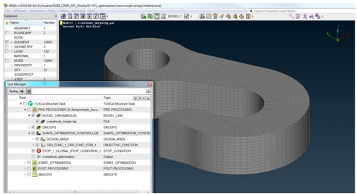
Optimizing the Cranehook Model (Tosca ANSA® environment) | ||
| ||
Define your design area that contains all regions which are allowed to be morphed.
To add a new MORPHING folder to your optimization task, right click on Tosca Structure Task and select :
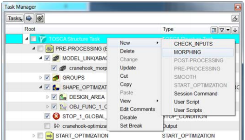
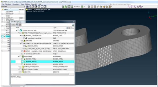
The MORPHING folder appears in Tosca Structure Task:

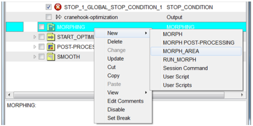
For each morphing area add a MORPH_AREA block via right-click on MORPHING folder:
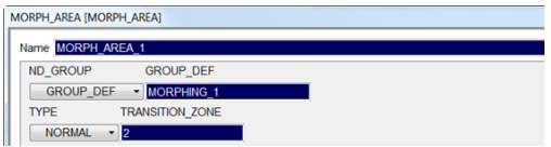
For each MORPH_AREA different properties can be defined. Define a name for your MORPH_AREA, here MORPH_AREA_1, then select under ND_GROUP the GROUP_DEF option. In GROUP_DEF, enter a ? and select or define a node_group describing the area to morph. Under TYPE, select the direction of the morphing displacements vectors. So far only NORMAL is supported Under TRANSITION_ZONE the number of nodes as transition zone can be entered:
Create the set of necessary MORPH_AREA definitions. The definitions can be highlighted interactively on the FE model:
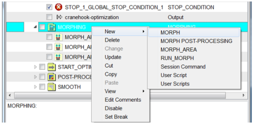
Add a new MORPH command via right-click on MORPHING folder and adding :
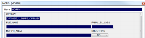
To link your MORPHING with a valid shape optimization task, do the following :
- Define a name in the pop-up window.
- Click in OPTIMIZE.
- Type ? and select your previously defined shape optimization, here OPTIMIZE_1_SHAPE_OPTIMIZATION_CONTROLLER
Note: All manufacturing and design variable constraints defined in this optimization task are considered during the morphing.
Select your MORPH_PARAM_FILE csv file to be executed. Then select the morphing areas:
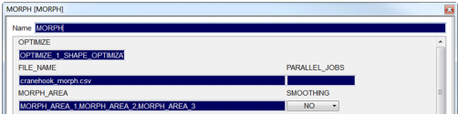
(optional) Define PARALLEL_JOBS and SMOOTHING:
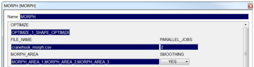
With PARALLEL_JOBS the number of parallel solver runs being started by Tosca Structure can be defined. E.g. 2 means that Tosca Structure runs always 2 FE solver runs in parallel (as long as enough morphing variants are available for calculation) SMOOTHING switches surface smoothing of nodes in modified morphing areas on/off.
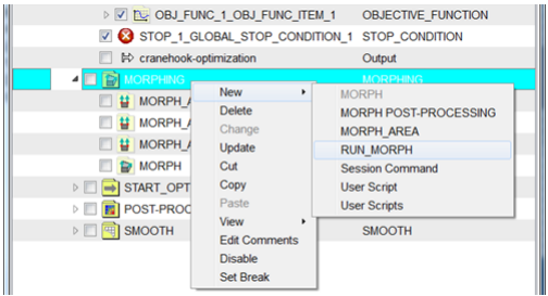
Run the morph task. Add a 'RUN_MORPH' command via right-click on MORPHING folder.
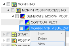
Create your visualization sequence using Tosca Structure.report in the same way like for shape optimization results: select your results using MORPHING | MORPH POST-PROCESSING | GENERATE_MORPH_POST_FILE | CONTOURPLOT and visualize with MORPHING | MORPH POST-PROCESSING | GENERATE_MORPH_ POST_FILE | MORPH_VTF_VISUALIZATION | VIEW:
The result looks as follows:
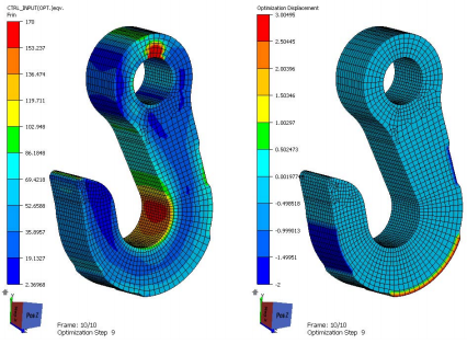
In the *.vtfx-File, you can see the controller input (f.e. stresses) and the nodal displacements for all experiments. Each frame corresponds to an experiment. In this example, the experiment 8 with the large-scale modification of the geometry gives the best results for the stresses. The experiment 9 which is a combination of grow and shrink gives good results too, and the modified geometry is significantly lighter than the geometry in the experiment 8. So the experiment 9 can be a good compromise for further processing (e.g. a subsequent local shape optimization...).